Overview

In this project, I implemented a mesh editor that can use either Bezier curves and surfaces or triangle meshes to represent 3D objects. The triangle mesh method also has upsampling so that there are more smaller triangles to better approximate the actual object. I liked how I could see two different ways of representing objects and the pros and cons of both. It was also interesting to see how big of a difference loop subdivision made in better representing the objects.

Section I: Bezier Curves and Surfaces

Part 1: Bezier curves with 1D de Casteljau subdivision

The de Casteljau algorithm is used to evaluate Bezier curves from control points. Each step of the algorithm evaluates a new set of points which are used in the successive step of the algorithm as the new control points. Eventually, the algorithm reduces the set of points to just one point, which is a point that lies on the Bezier curve for a given paramter t. Different values of t will yield different points on the curve.

My implementation generates a new point by linearly interpolating consecutive points of the control set with the parameter t. These new points are stored and returned. Future steps of the algorithm used this returned set of points as the new control set until only one point remains.

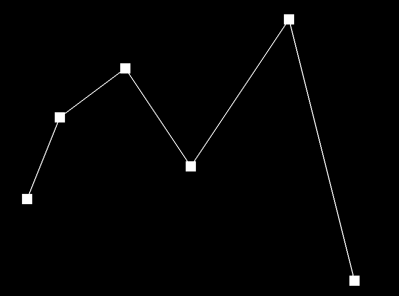
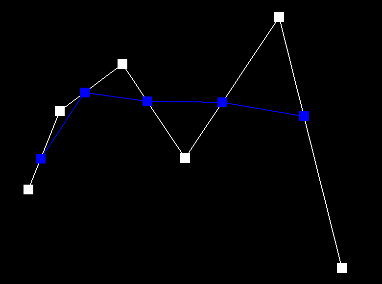
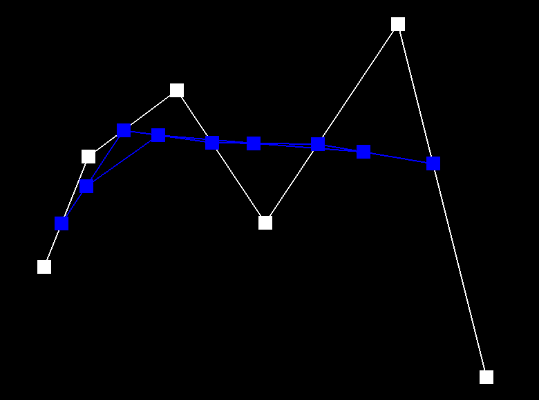
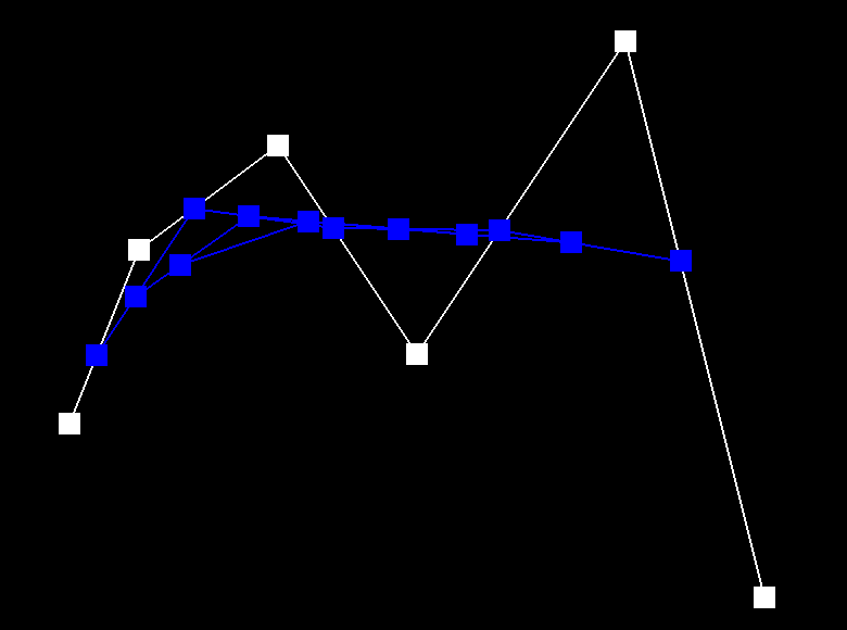
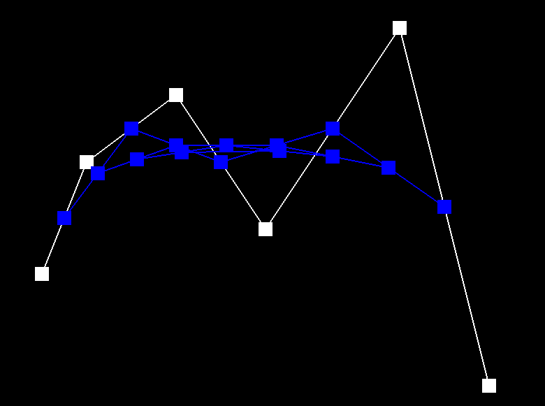
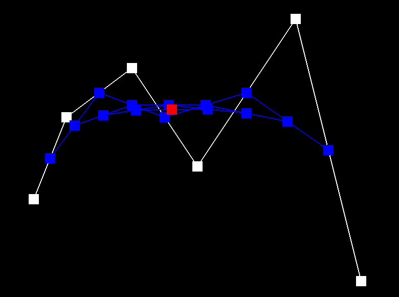
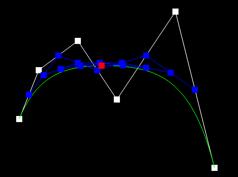
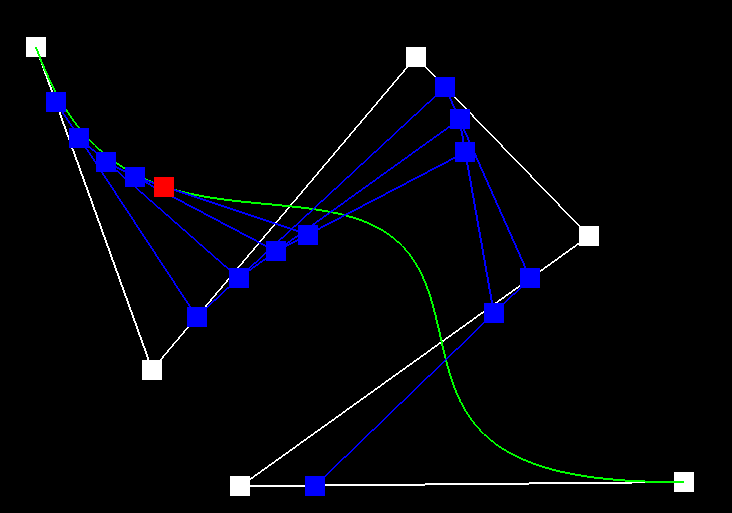
Below depicts the process of de Casteljau's algorithm. We start with the six control points and each step interpolates a new set of blue points. After step 5, the set of six points is reduced to a set of one point, which is a point that lies on the Bezier curve (green). The last image is a Bezier curve with different control points and parameter t.

Part 2: Bezier surfaces with separable 1D de Casteljau subdivision

De Casteljau's algorithm extends naturally from 2D curves to 3D surfaces. A Bezier surface is made up of Bezier curves going in the same direction. The points on the curves for a given parameter u are used as the control points for the Bezier curves that run in the opposite direction. The points on these perpendicular curves are interpolated with another parameter u. The criss-crossing of Bezier curves creates a Bezier surface, approximating the desired surface.

My implementation evaluates Bezier surfaces by evaluating patches of the surface. A point on the Bezier patch with parameter u and v is evaluated by first evaluating the Bezier curves that run along the same direction with u. Each curve has it's own set of control points, and is evaluated the same way as part 1 above, using the same u for all curves. Then, the evaluated points on each of these curves is the new set of control points for the final Bezier curve that runs perpendicular to the original curves. The final point is interpolated using de Casteljau's algorithm with the new control points and v.

Section II: Sampling

Part 3: Average normals for half-edge meshes

My implementation builds the normal vector of the vertex by summing the weighted normal vectors of each incident face to the vertex. The weighted vector of a face is the normal vector of the face multiplied by the area of the face. The weighted vectors are summed together into one vector, which is then normalized to obtain the vertex normal vector.

Given a halfedge H, the vertices of the next (clockwise order) face are the central vertex, the source vertex of H->twin, and the source vertex of H->twin->next->twin. If the twin is not a boundary edge, we find the area of the face by taking half the cross product of two of the edges of the face, which gives us the weight of the face normal vector. If it is a boundary edge, we continue the process to the next face without calculating the area. The algorithm stops adding the weighted vectors to the vertex normal when we reach back to the original halfedge. Finally, we normalize the vertex normal.

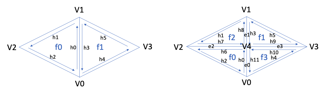
Part 4: Half-edge flip

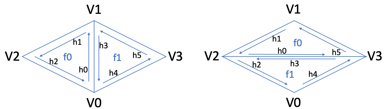
My implementation reassigns pointers according to the diagram below. On the left is the layout of two triangles before an edge flip. The right shows the layout of halfedges, vertices, and faces after flipping the middle edge. Edge flipping is done by modifying the mesh element attributes of each halfedge according to the diagram below. After halfedges are modified, the halfedge attribute of each face is reassigned to ensure correctness. For example f0's halfedge is set to h0 and f1's halfedge is set to h3. Finally, the halfedge attribute of each vertex is reassigned.

Part 5: Half-edge split

My implementation reassigns pointers according to the diagram below. On the left is the layout of two triangles before an edge split. The right shows the layout of halfedges, vertices, edges, and faces after splitting along the middle horizontal. Edge splitting is done by modifying the mesh element attributes of each halfedge according to the diagram below. After halfedges are modified, the halfedge attribute of each face, vertex, and edge is reassigned to ensure correctness. For example f0's halfedge is set to h0 and f1's halfedge is set to h3. Finally, the position of the new middle vertex is calculated using lerp with two opposite points and a parameter of 0.5.

Series of Splits Alternating flipping and splitting

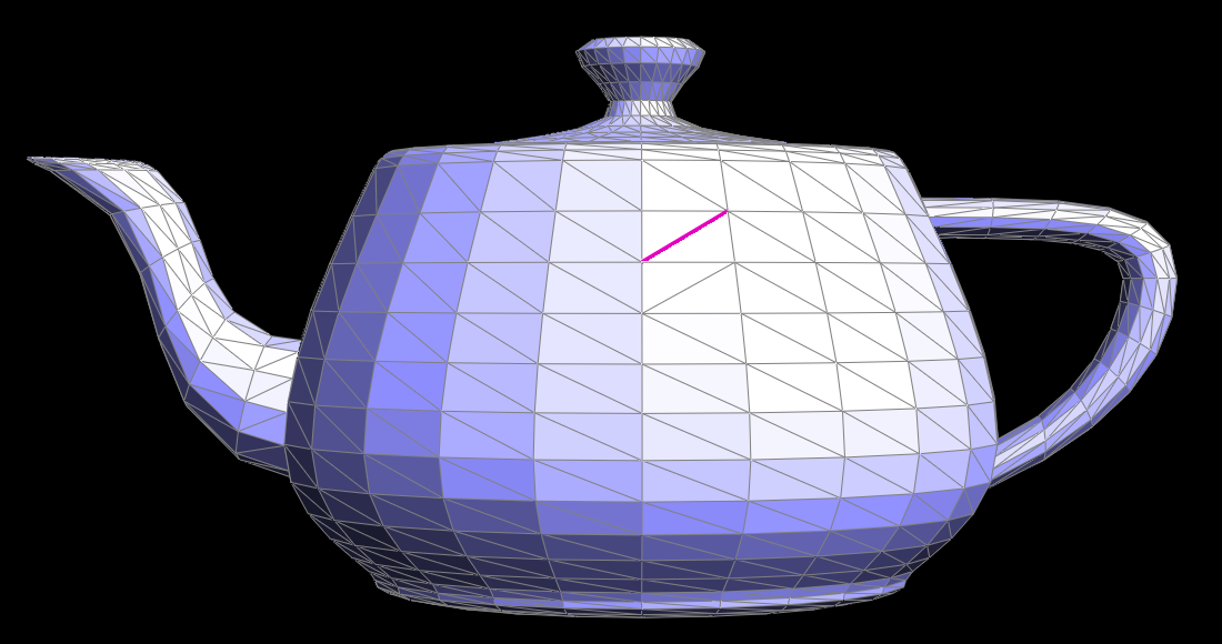
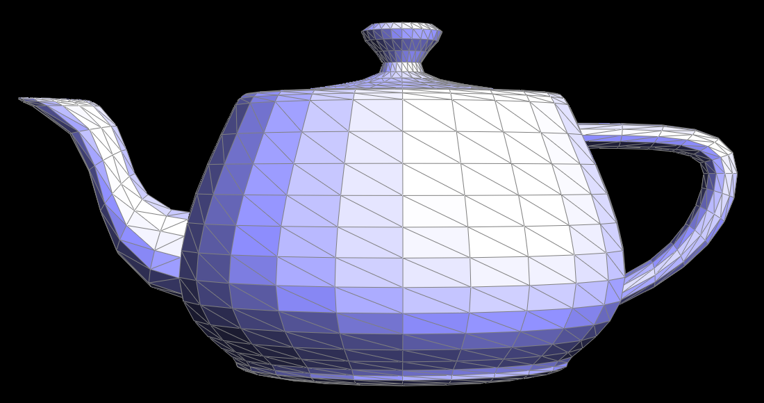
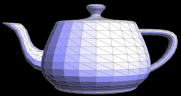
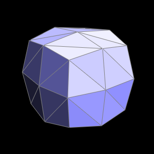
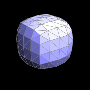
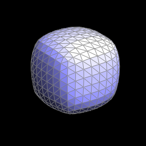
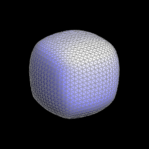
Part 6: Loop subdivision for mesh upsampling

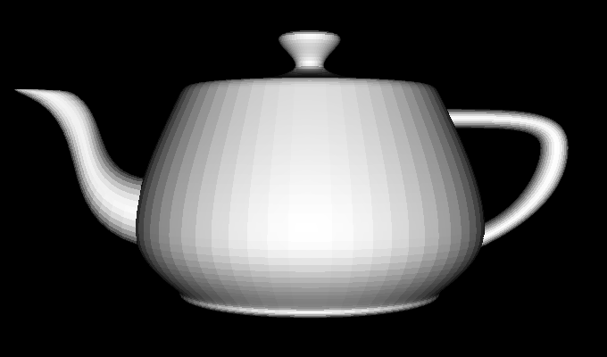
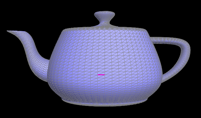
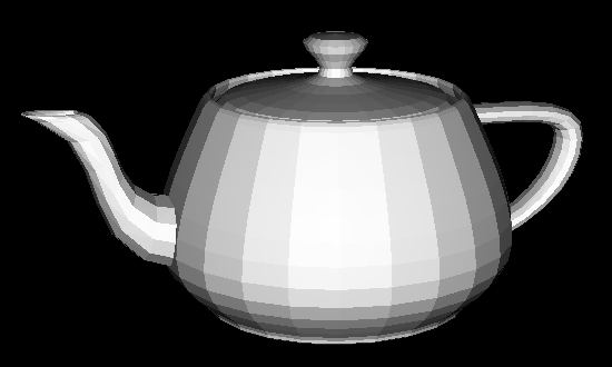
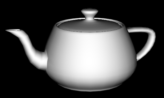
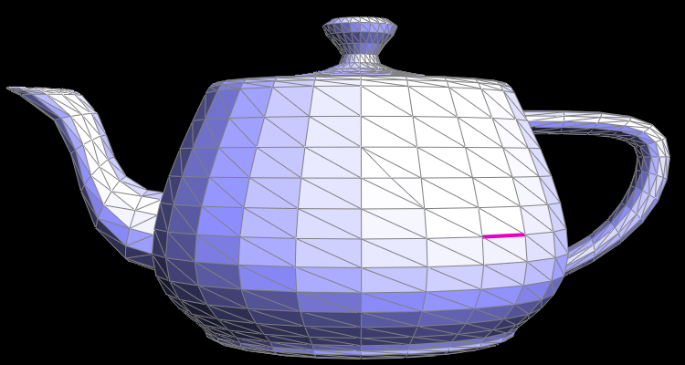
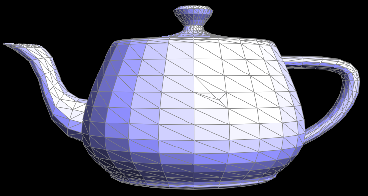
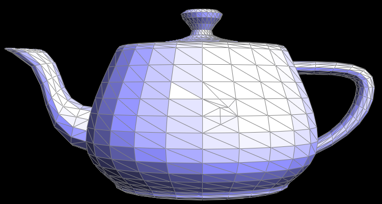
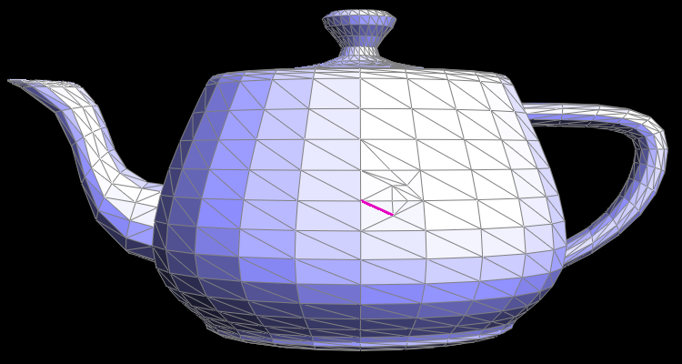
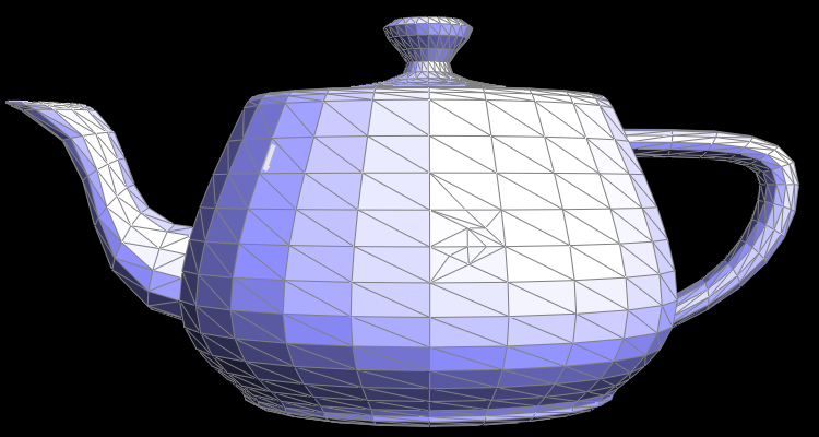
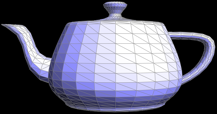
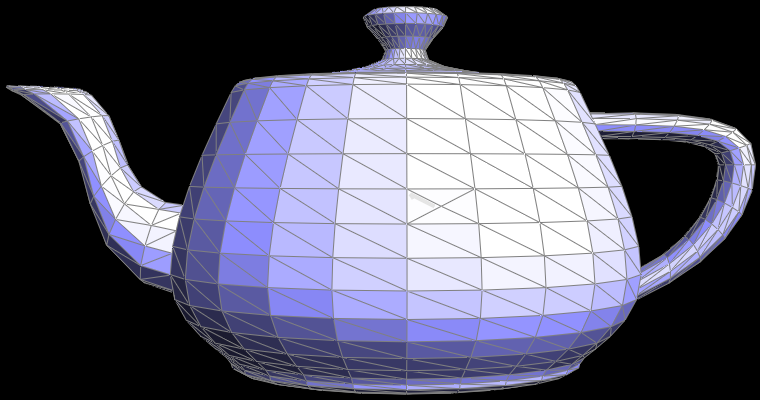
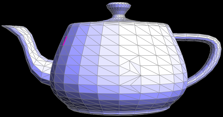
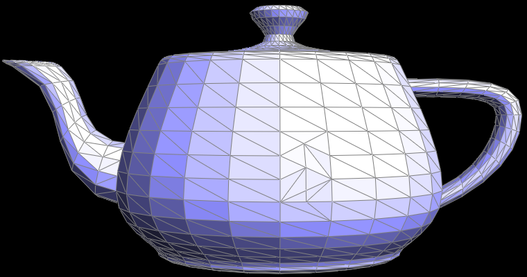
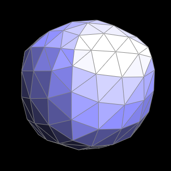
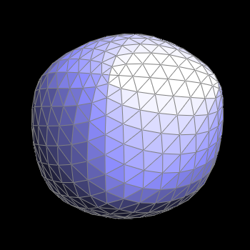
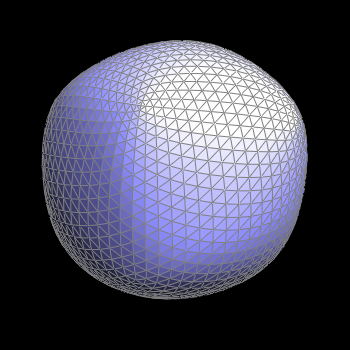
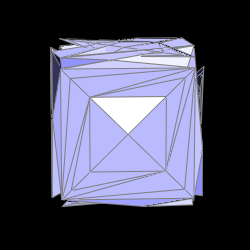
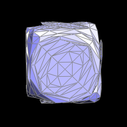
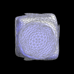
My upsampling implementation first precomputes the new positions of the new and old vertices. The new position of a new vertex is stored with the edge the new vertex will lie on. The new position of an old vertex is calculated by looping through each of it's neighboring vertices, applying some weights, and storing the new position with the old vertex. The actual position isn't updated until the end so that the splitting can be done on the old positions. The upsampling process then divides each triangle into four subtriangles. For each edge, if both end vertices are old, then the edge is split, and the new vertex that is created gets assigned the new position that's stored with the split edge. When an edge is split, the new edges and vertices are flagged as new so that the upsampling method knows which edges to split, flip, and skip. Also, if the edge is new, and strictly one end vertex is new, then the edge is flipped. At the end of one subdivision loop, all edges and vertices have their new flag reset so the next iteration treats the updated mesh as the original mesh.

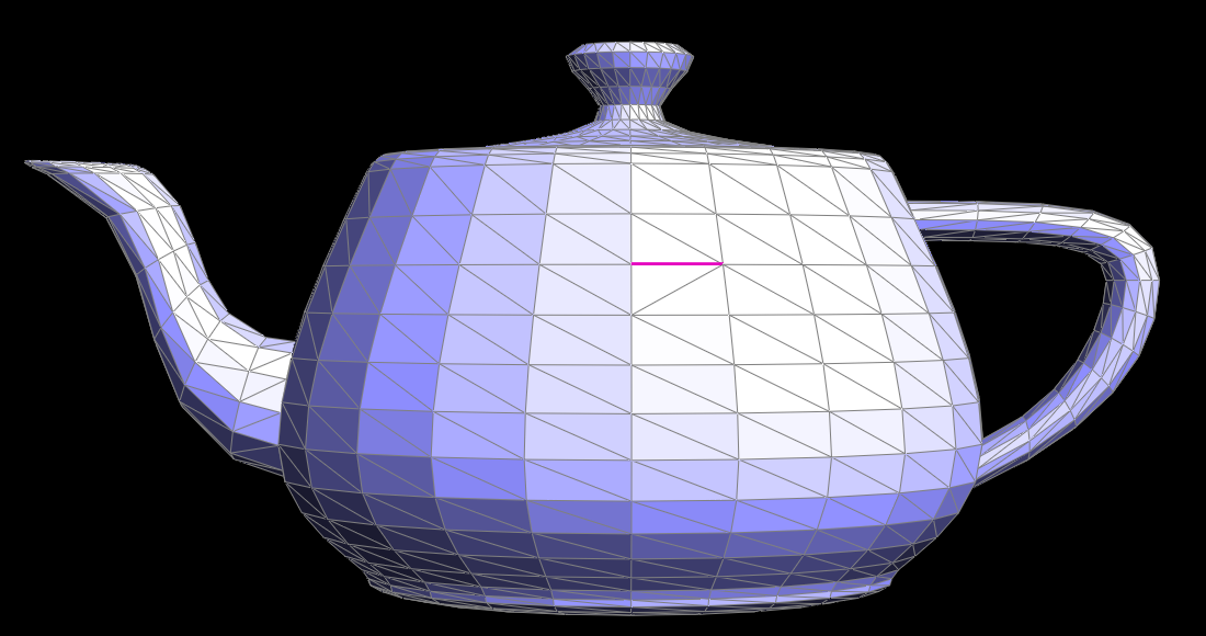
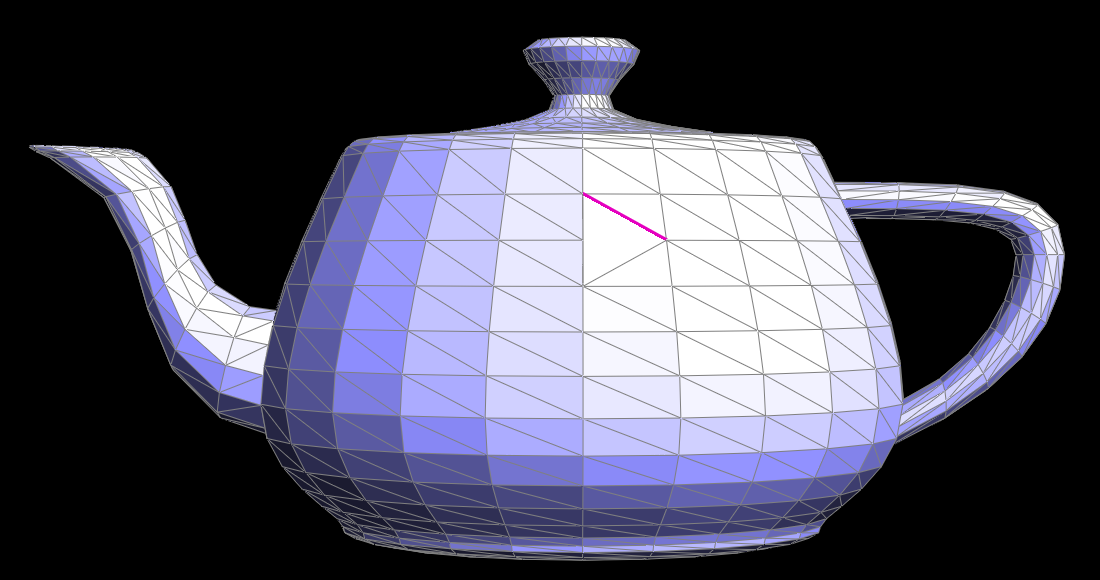
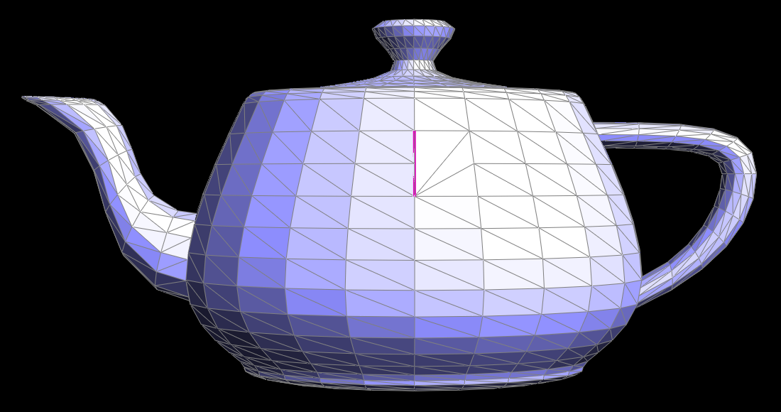
After loop subdivision, the mesh becomes less blocky because the desired surface is now represented by more elements, and so angles and curves are better approximated. Sharp corners and edges become rounded out because of the vertex position updates. Even if the original shape should have a sharp edge or corner, the subdivision causes the shape to round out.

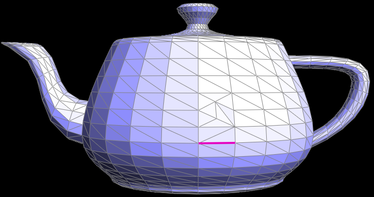
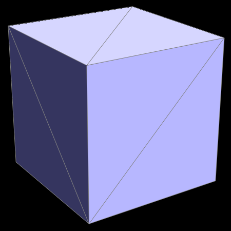
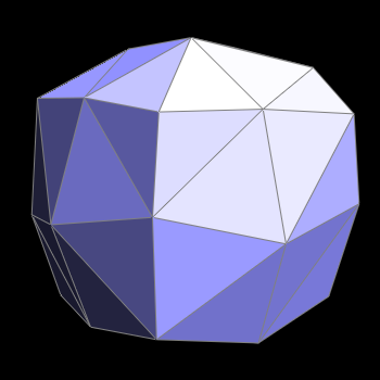
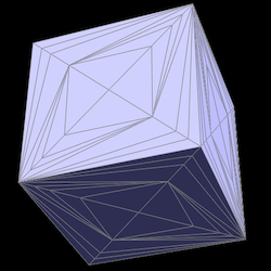
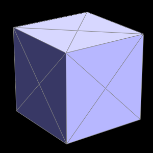
This rounding effect can be reduced by pre-splitting some edges. Splitting edges so that there are more vertices concentrated around the sharp corners and edges will reduce the rounding effect when upsampling. This is because there will be more vertices along sharp edges and corners to weigh the new positions of the old vertices. Below is an example on the cube:

The cube also has an issue of looking assymetric after upsampling. This is because each face of the original cube has one edge across the face connecting two opposite vertices. However, the other two opposite vertices are not connected. This results in some vertices having degree five and other having degree four. The position of a vertex with degree five will be moved more than a vertex with degree four because the position of the higher degree vertex is weighted by five vertices instead of four. Thus, the five degree vertex will move more towards the center of the cube compared to a four degree vertex, resulting in assymetry. This can be corrected by splitting each cube face's edge so that both pairs of opposite vertices are connected. The preprocessing ensures that all vertices have the same degree so that their positions will be updated the same amount.