In this project, I implemented a simple ray tracer. Specifically, I implemented ray generation and scene intersection tests in the first part. Next, to render images more efficiently, I built a BVH along with the bounding box intersection tests. In the third and fourth part, I worked on implementing complex shading and lighting, combining bsdf's, different sampling methods, and multibouncing of light rays to realistically render objects and scenes. Lastly, I optimized the program by adding adaptive sampling so that images can render even faster without losing image quality. Overall it was a really fun project, and seeing the rendered images improve from stage to stage was really satisfying.
Part 1: Ray Generation and Intersection
In the rendering pipeline, each pixel is updated with the average spectrum of ns_aa random rays going through the pixel. Each ray is determined by a random normalized image coordinate inside the pixel. This coordinate is mapped to the same proportional location on the sensor in camera space. The vector from the camera source to the mapped location is the direction vector in camera space which can be translated into a direction vector in world space using the camera to world tranform. The generated ray has origin at the camera position in world space and direction of the tranformed direction vector. We also generate the ray with min and max lengths to make object depth ordering easier later on.
This part also involves finding ray-triangle intersection and ray-sphere intersection. Ray-object intersection is computed for every ray in estimating one of the spectrums in the pixel.
Specifically for ray-triangle intersection, I used the Moller Trumbore algorithm. This algorithm takes as input the triangle's vertices, the ray origin, and the ray direction to find if there is an intersection. It's more optimized because it doesn't have to calculate the plane the triangle is lying on and then check if the intersection between the ray and the plane is in the triangle. It outputs the distance t of intersection, and b2 and b3 which are barycentric coordinates for v2 and v3. If there is a valid intersection (eg. t>=0, all b's are in [0,1], t < ray max_t) then we store information regarding the intersection (t, surface normal, bsdf, the current object) and update the new max limit of our ray.
Ray-sphere intersection is similar to ray-triangle intersection except the method for checking for an intersection involves finding the t values that result in points on the ray that are a radius distance away from the center of the sphere. This process involves solving a quadratic equation, and uses the ray's origin and direction, as well as the sphere's center and radius. In solving the quadratic equation, if the discriminant is negative, there is no intersection. If the discriminant is 0, there's one intersection. Otherwise, there are two. We're most interested in the intersection with smaller t-value because that's where our ray hits the sphere first. We also do similar checks to make sure our t-values are valid. In calculating the surface normal, we subtract the point of intersection from the origin of the sphere. Lastly we store information regarding the intersection and update the max limit of our ray with the first t value.
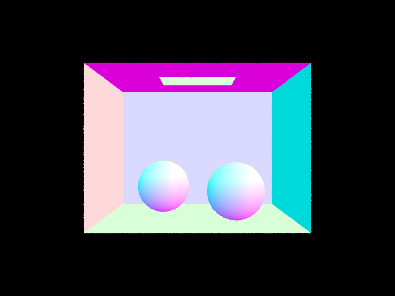
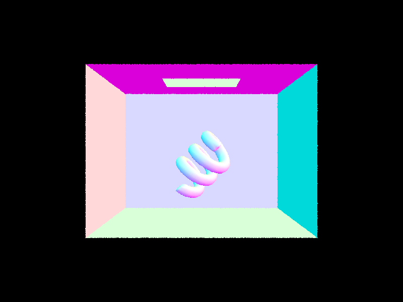
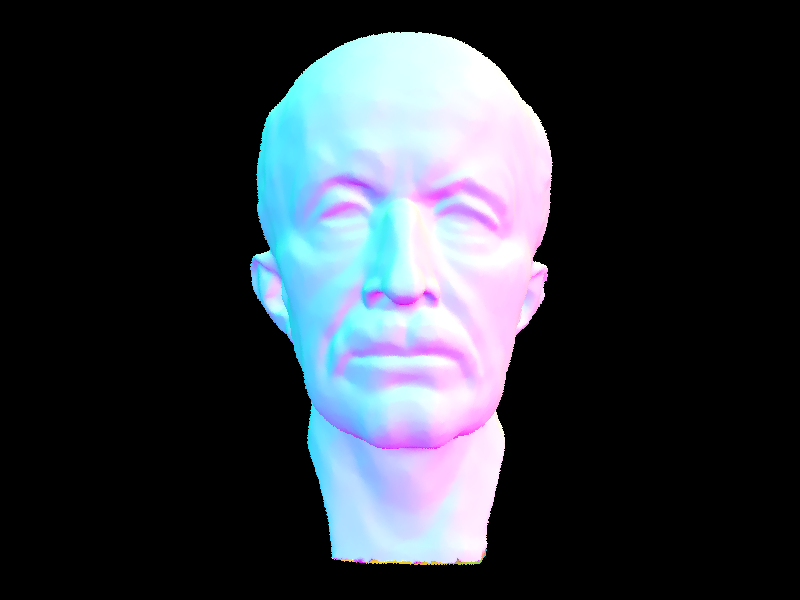
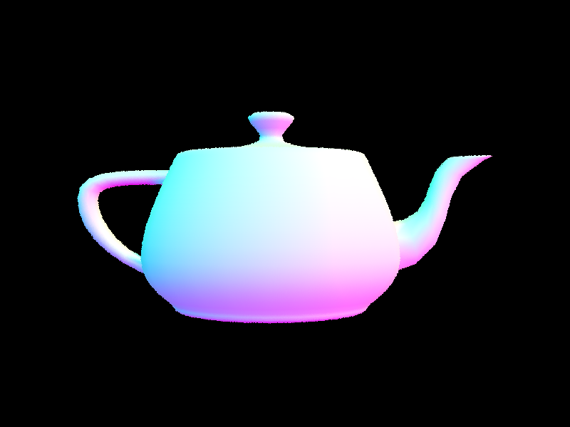
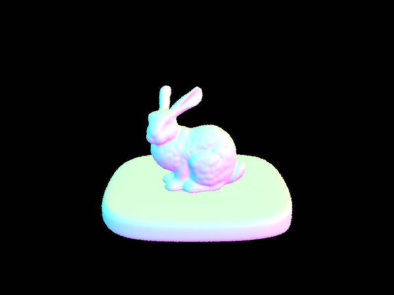
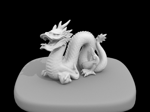
Here are some images with normal shading:
|
|
|
|
Part 2: Bounding Volume Hierarchy
My BVH algorithm finds splits by taking the average position of centroids of the bounding boxes. It then simulates a split along the x, y, and z axes given by the average position, and counts how many objects are split for each axis. The axis that splits objects most evenly is chosen as the split axis. The primitives are then grouped based on this split into a left and right group. These left and right groups are passed down to the recursive calls for generating the left BVH node and the right BVH node, respectively.
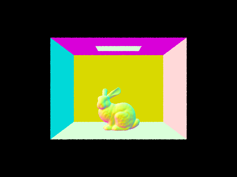
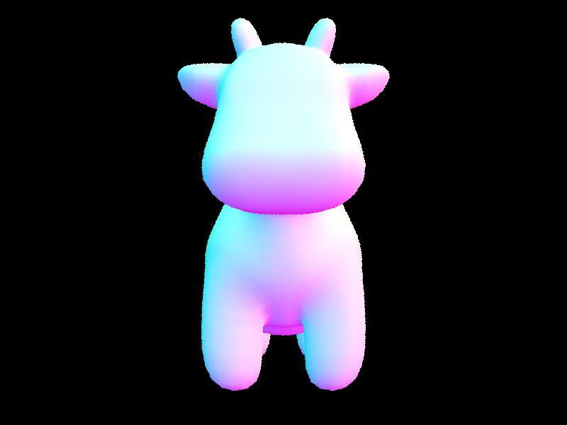
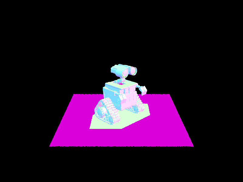
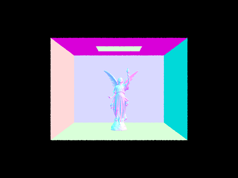
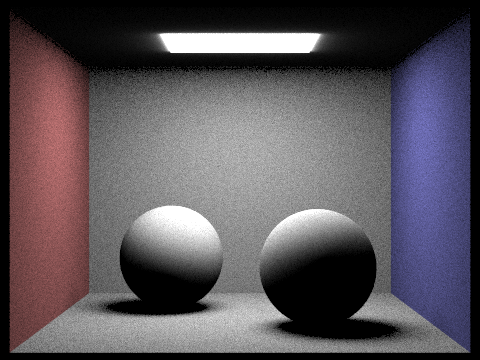
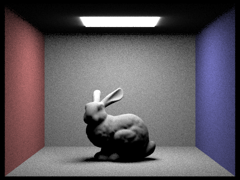
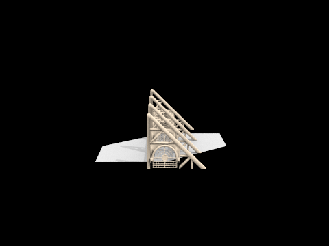
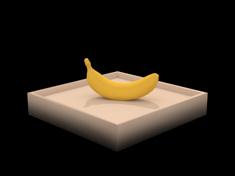
Here are some complex images rendered with BVH:
|
|
|
|
Let's compare rendering times with and without BVH. Rendering teapot.dae single-threaded on the hive machines without BVH takes 22.3344 sec. Rendering it with BVH takes 0.4603 sec. Eight-threaded without BVH takes 19.1847 sec. Eight-threaded with BVH takes 0.1017 sec.
Rendering cow.dae with a single thread without BVH takes 57.4317 sec. Rendering it with BVH takes 0.3076 sec. Using eight threads without BVH takes 41.2491 sec. Using eight threads with BVH takes 0.065 sec.
Rendering bunny.dae single-threaded without BVH takes 537.4716 sec. Rendering it with BVH takes 0.5948 sec. Eight-threaded without BVH takes 264.8468 sec. Eight-threaded with BVH takes 0.1323 sec.
As we expect, BVH dramatically decreases rendering times since it runs in logarithmic time compared to linear for no BVH. Rendering with BVH is further taken advantage of with multithreading.
|
|
|
Part 3: Direct Illumination
The first way of calculating direct illumination is by sampling light uniformly around a hemisphere at each point. A vector around a hemisphere is randomly sampled, then transformed into world space, then used to create a ray starting at the hit point. The hit point is always the same because this is the hit point of our camera ray to an object, but the ray is random because the direction is given by the randomly sampled vector. If the ray intersects a light source first, then we update the light calculation according to the reflectance equation (by adding the total light so far with the product of emission of the light source, diffuse reflectance, and the cos of the angle between the incoming vector and normal vector). We lastly multiply this amount by 2 pi and average by dividing by the number of samples we took.
The second way of calculating direct illumination is by importance sampling light sources. For every light source, we sample rays from the hit point to the light source. If the light source is a point light source, we only sample once. If the ray does not intersect any other objects, we consider it the ray's origin (the hit point) to be in the path of the light source, and we update the total light according to the reflectance equation. This is adding the product of the light source's emission, the diffuse reflectance, and the cos of the angle between the incoming vector and normal vector, divided by the pdf of the sampler. Lastly we average the total by dividing by the number of samples.
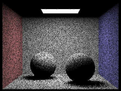
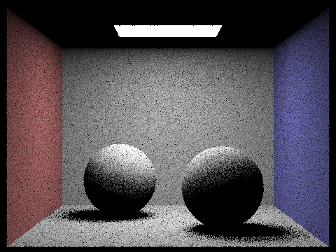
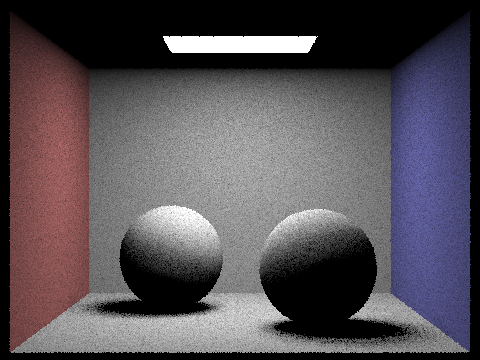
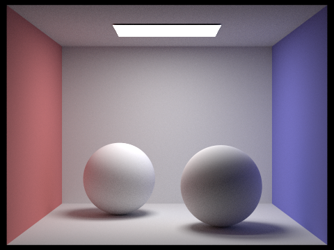
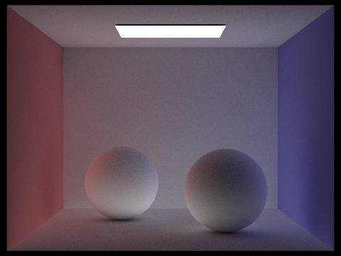
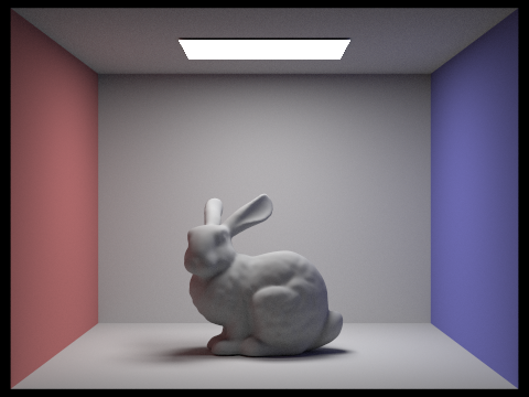
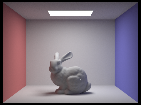
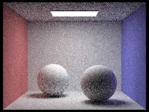
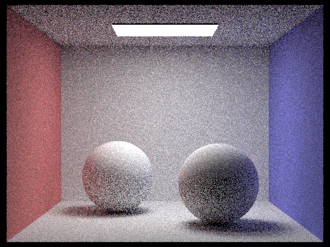
Below shows four renderings. The top row is rendered using uniform hemisphere sampling, and the bottom row is rendered with importance sampling of the light sources. All images are rendered with 64 samples per pixel and 32 samples per light.
|
|
|
|
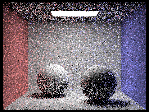
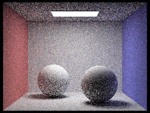
We now look at the effect the number of samples per light has on the image. With lower levels of samples per light, the soft shadows in the image become much noiser. This is because if we only have a few number of samples to sample the light, some or all of those samples could not hit the light source. This results in a black spot even though the dark spot can partially see the light source. It also results in an equally bright spot for two points that see different amounts of light. These cause the soft shadows to be noiser instead of smooth and soft because we don't get the same gradient from black to white as we do when we can take more smaples. In other words, the shadows are not approximated as well when we have fewer samples because we aren't able to reach the exact amount a point sees the light source.
|
|
|

|
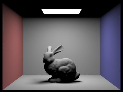
Now we compare uniform hemisphere sampling and importance sampling of light sources. The first thing that stands out is the graininess of the image rendered using hemisphere smampling. The overall scene isn't as smooth as the importance sampling version. This is expected because in hemisphere sampling we don't always sample light sources, so it's possible that all of our samples for a single hit point misses the light, which results in a dark spot causing the grain. Furthermore, there is more glare in the image with uniform hemisphere sampling, both on the bunny's ears and especially coming from the edges of the ceiling light. Lastly, the shadows in the importance sampling image are much smoother and more realistic, a direct result of being able to sample only light sources to reduce the grain and noise.
|
|

|
Part 4: Global Illumination
For indirect lighting, we need to recursively find the value of a pixel by tracing the rays through their multiple intersections. We begin with the ray and the first intersection. The ray's depth at the beginning is 0. We first calculate the one_bounce_radiance of the ray at the intersection and add this to our running total. Next, two conditions need to be met to continue the ray tracing. The first is if the ray's depth is less than the max ray depth parameter. The second is if a random number between 0 and 1 is less than our continuation probability of 0.65. If both conditions are met, then we continue calculating the radiance. We sample a random vector from the hit point, and build our next ray starting at the hit point with the sampled vector's direction, and initialize the ray's depth one level higher than our previous ray. If this new ray intersects something, we continue the recursion and calculate the radiance according to the reflectance equation. We add the product of the emission of the original intersection, the radiance of our new ray, and the cos of the angle between the incoming vector and the surface normal, divided by the pdf and the continuation probabilty, to our running total. In calculating the radiance of the new ray, we recursively call this radiance function.
|

|
|

|
|

|
|
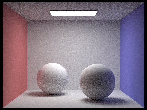
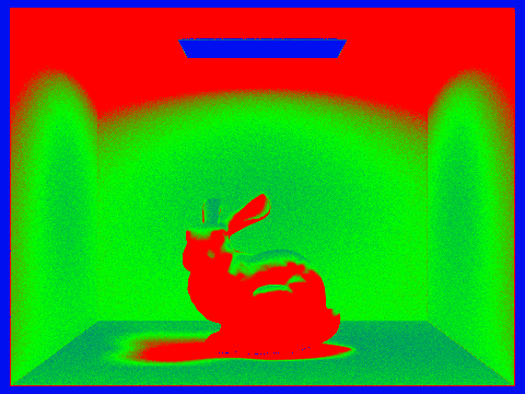
We can use the images above to understand how global illumination is decomposed into direct and indirect illumination. In direct illumination only, we're able to easily see the defined shapes and shadows. Also, things are quite smooth. In indirect illumination only, objects aren't as defined and the primary light source doesn't refelct much, but we're able to see the effect of multiple bounce lighting. For example, we can see the different colors of the walls being reflected onto other walls and the spheres in the middle. Combining these two yields the global illumination image.
|
|

|
|

|
At max_ray_depth=0, we get the same effect as direct illumination because we are not allowing our rays to bounce at all. We begin seeing the effect of indirect illumination at max_ray_depth=2. We can see the red and blue colors of the wall reflecting off the other objects. At 100 max ray depth, we don't see much compared to when max ray depth is 3. Since light dissipates quickly after multiple bounces, a super high max ray depth isn't going to make a large difference so we can just render something less expensive for similar results. Also since we're using Russian Roulette path termination, it's almost impossible our path is going to bounce 100 times anyways.
|
|
|
|

|
|

|
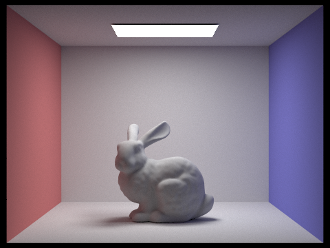
Now we compare images with different number of samples per pixel. We get pretty grainy images starting from 1 sample per pixel to 16 samples per pixel. After that the images become a lot smoother and with 1024 the image is extremely smooth. There's a huge difference when sampling with a low number of samples per pixel compared to when sampling with a large number of samples per pixel. The better results are definitely worth the extra rendering costs.
Part 5. Adaptive Sampling
Adaptive sampling is a method of sampling that tries to minimize the amount of sampling while maintaining image quality. As a pixel is being sampled, if the pixel illuminance has converged under a threshold, then the program will stop sampling for that pixel. This is so that our renderer won't spend equal time on pixels that quickly converge.
In my implementation, as we're ray tracing for a pixel, we keep track of the sum of spectrums' illuminance so far (s1) as well as the sum of the squares of the spectrums' illuminance (s2). Every batch number of samples (eg. 64), we test if the pixel has converged. We first calculate the mean and the variance of the pixel's illuminance for the number of samples taken so far (n):
mu = s1 / n
variance = 1 / (n - 1) * (s2 - s1^2 / n)
I = 1.96 * sqrt(variance / n)
Next, if I (calculated in the last line) is less than our maxTolerance * mu, the pixel has converged with 95% confidence and we can stop sampling for that pixel. The max tolerance is a parameter and defaults to 0.05.
|
|