|
|
|
|

|
|
|
In this project, I extended the PathTracer implementation to be able to render different materials and surfaces. I started by implementing BSDF for mirror and glass materials, and then worked on rendering objects that have microfacets. This project involved understanding various physical properties of different materials and specifically how light interacts with them. The results are nicely rendered images that closely resemble the real world.
In this part I implemented sampling and BSDF for mirror and glass materials. Surfaces that are mirrors reflect light, so an incoming vector w_i has to be reflected across the normal of the surface. This is done by negating the x and y components of the vector. Sampling from a mirror is also straightforward as it's just the reflectance of the surface divided by the cos angle of the incoming vector w_i.
For glass materials, we have to also implement refraction. We use Snell's Law to calculate the refractance direction. The eta term used in Snell's Law is determined by the action of the incoming vector. If we are entering the surface, we use the inverse of the index of reflection. Otherwise, we use the index of reclection. We also test for total internal reflection to see if there is any refraction. As for sampling the glass BSDF, when we have total internal reflection, we treat this case as having reflection like a mirror. Otherwise, we use Schlick's approximation to approximate the result of using Fresnel equations. We use Schlick's reflection coefficient to determine if we have reflection or refraction.
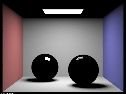
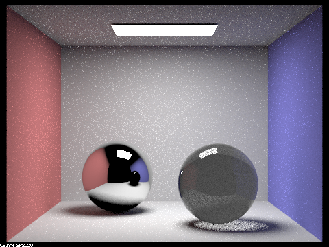
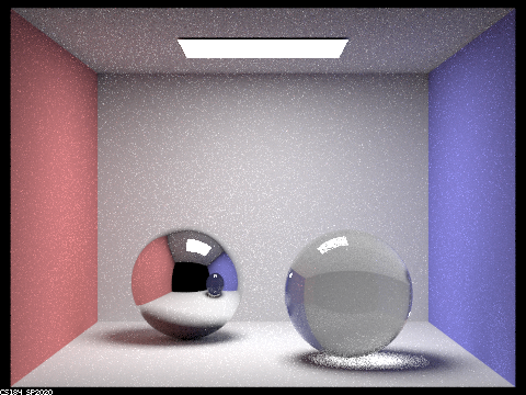
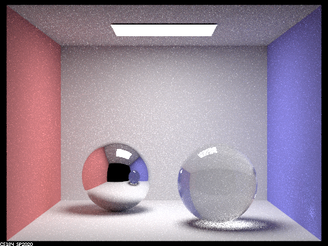
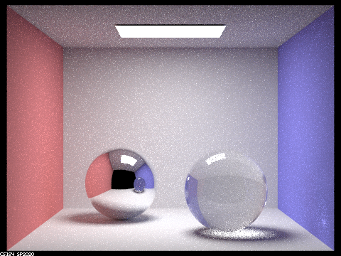
Here is a sequence of images with varying max ray depth. The sphere on the left is a mirror and the sphere on the right is glass. All images are rendered with 64 samples per pixel and 4 samples per light.
|
|
|
|
|
|
|
|
|
|
When the max ray depth is 0, we only see the area light because we are only capturing light that directly reaches the camera. At max ray depth 1, we have one bounce effects, so we are only able to see direct illumination. When max ray depth is 2, we can see the walls being reflected off the mirror sphere and a little bit on the glass sphere. This is light hitting the wall then hitting the spheres and then finally reaching the camera. Next at max ray depth 3, we can finally start to see the glass sphere refracting light, since the light has to go through the ball when it's refracted. At max ray depth 4, the reflection of the glass sphere in the mirror sphere has color, because an iditional bounce is able to capture the light that hits the blue wall and the is refracted through the glass ball. We also see a shiny spot on the edge of the blue wall for similar reason. Max ray depth 5 has similar features to max ray depth 4, but is a little brighter due to more opporunities for light to bounce, brightening up the scene. At max ray depth 100, there are no significant changes.
In this part, I implemented the Microfacet model for isotropic rough conductors that only reflect. The Microfacet BSDF is evaluated by multiplying together the Fresnel Term, the shadowing-masking term, and the normal distribution function, and then dividing by the dot product of the normal with the outgoing vector, the dot product of the normal with the incoming vector, and the constant 4. For the normal distribution function, we use the Beckmann distribution. For the Fresnel term, we approximate the actual air-conductor Fresnel term by calculating the Fresnel terms for RGB channels seperately for each channel's fixed wavelength. Lastly, we importance sample the Beckmann NDF to get a sample for the Microfacet BSDF. To sample, we choose a random number between 0 and 1, then reverse sample the CDF for the provided pair of pdfs for the Beckmann NDF. From this we have a sampled theta and phi angle, and we can then convert these spherical coordinates to cartesian coordinates to find the half vector h. Next, we reflect wo over h to get wi, and calculate the pdf of wi. Lastly, we return the BSDF spectrum value with wo and wi. In practice, we check if wi and wo are valid by making sure dot(n, wi) and dot(n, wo) are positive. In the case they are invalid, the pdf is 0.
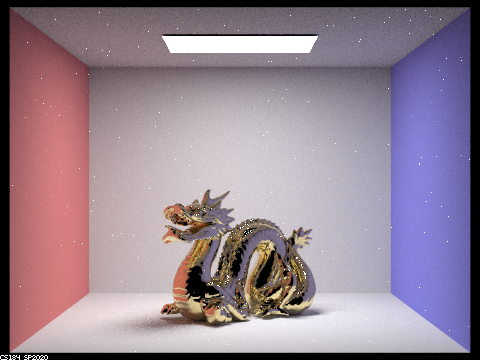
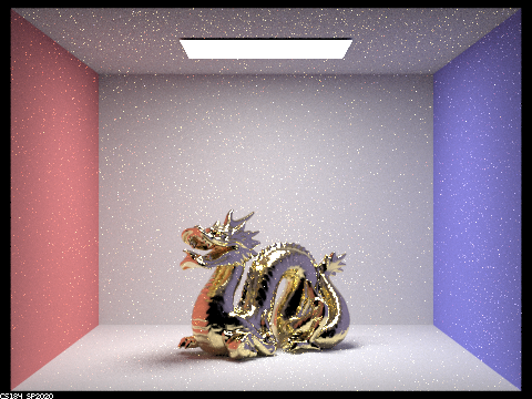
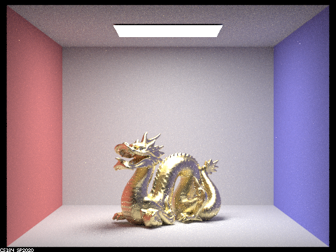
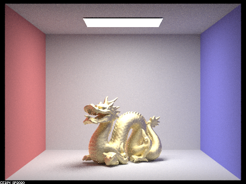
Below we display the effect of the roughness coefficient α in the normal distribution function. Notice the dragon's gold surface change in appearance as α changes. As α increases, the surface becomes rougher and diffuses light more evenly. When α is small, the surface is smoother and has a more glossy look because there is more reflection. All images are sampled with 128 samples per pixel, 1 sample per light, and have a max ray depth of 5.
|
|
|
|
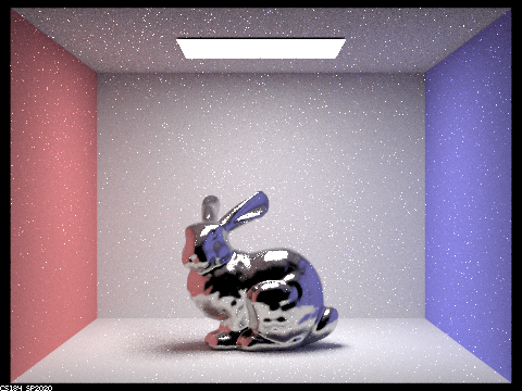
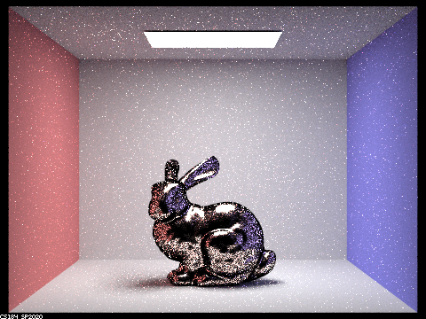
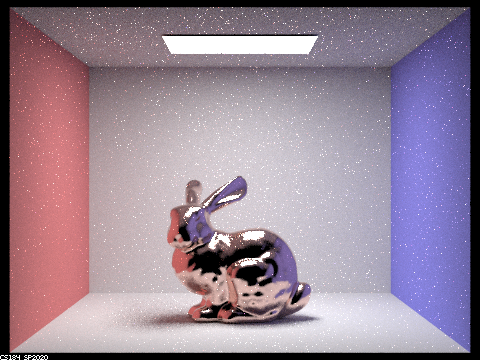
Here are two images of CBbunny in copper. The left version is sampled with cosine hemisphere sampling and the version on the right uses importance sampling. With importance sampling we're able to get much less noise in our image, because we are directly sampling in the direction of light rather than random directions around a hemisphere. These were sampled with 64 samples per pixel, 1 sample per light, and have a max ray depth of 5.
|
|
Lastly, we render the same CBbunny but in cobalt. The cobalt bunny has very similar specular properties to the copper bunny, probably because cobalt and copper are pretty similar. At least the color is different. To change the metal, I used this website to look up the refractive index (η) and extinction coefficient (k) of cobalt at the fixed wavelengths for the R,G,B channels. Parameters listed below.
R (614 nm): η=2.1849, k=4.0971
G (549 nm): η=2.0500, k=3.8200
B (466 nm): η=1.7925, k=3.3775