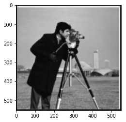
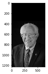
cameraman.png
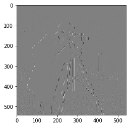
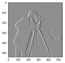
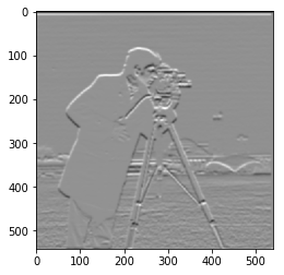
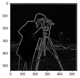
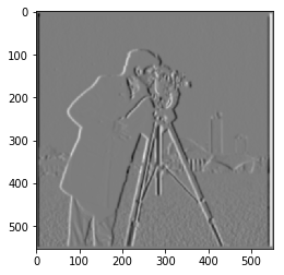
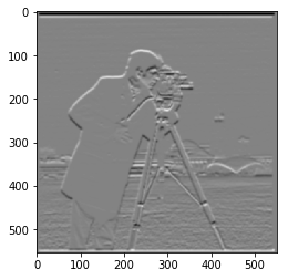
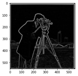
Let Dx=[1 -1], Dy=[1 -1].T. The partial derivative of the image with respect to x is found by convoluting the image with Dx. The partial derivative of the image with respect to y is found by convoluting the image with Dy. The gradient magnitude is found by taking the square root of the sum of the squares of both partial derivatives.
cameraman.png
Gradient w.r.t x
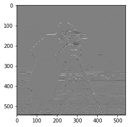
Gradient w.r.t y
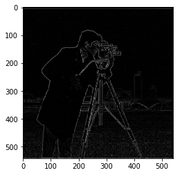
Magnitude of Gradient unfiltered
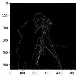
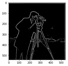
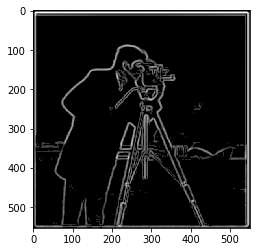
Magnitude of Gradient filtered (> 0.28)
The Gaussian filter hass size=12 and sigma=2. Image after blurring:
blurred cameraman.png with gaussian filter
Two Convolutions:
Gradient w.r.t x
Gradient w.r.t y
Magnitude of Gradient unfiltered
Magnitude of Blurred Gradient filtered (> 0.03)
Already we can see that the edges are clearer and the picture overall has less noise because of the initial blurring with the Gaussian filter.
Below is the single convolution method, done by taking the derivative of the filter w.r.t x and y, and then convoluting the image with the resulting DoG filter:
Gradient w.r.t x
Gradient w.r.t y
Magnitude of Gradient unfiltered
Magnitude of Blurred Gradient filtered (> 0.03)
The final filtered images of both methods look the same, as expected.
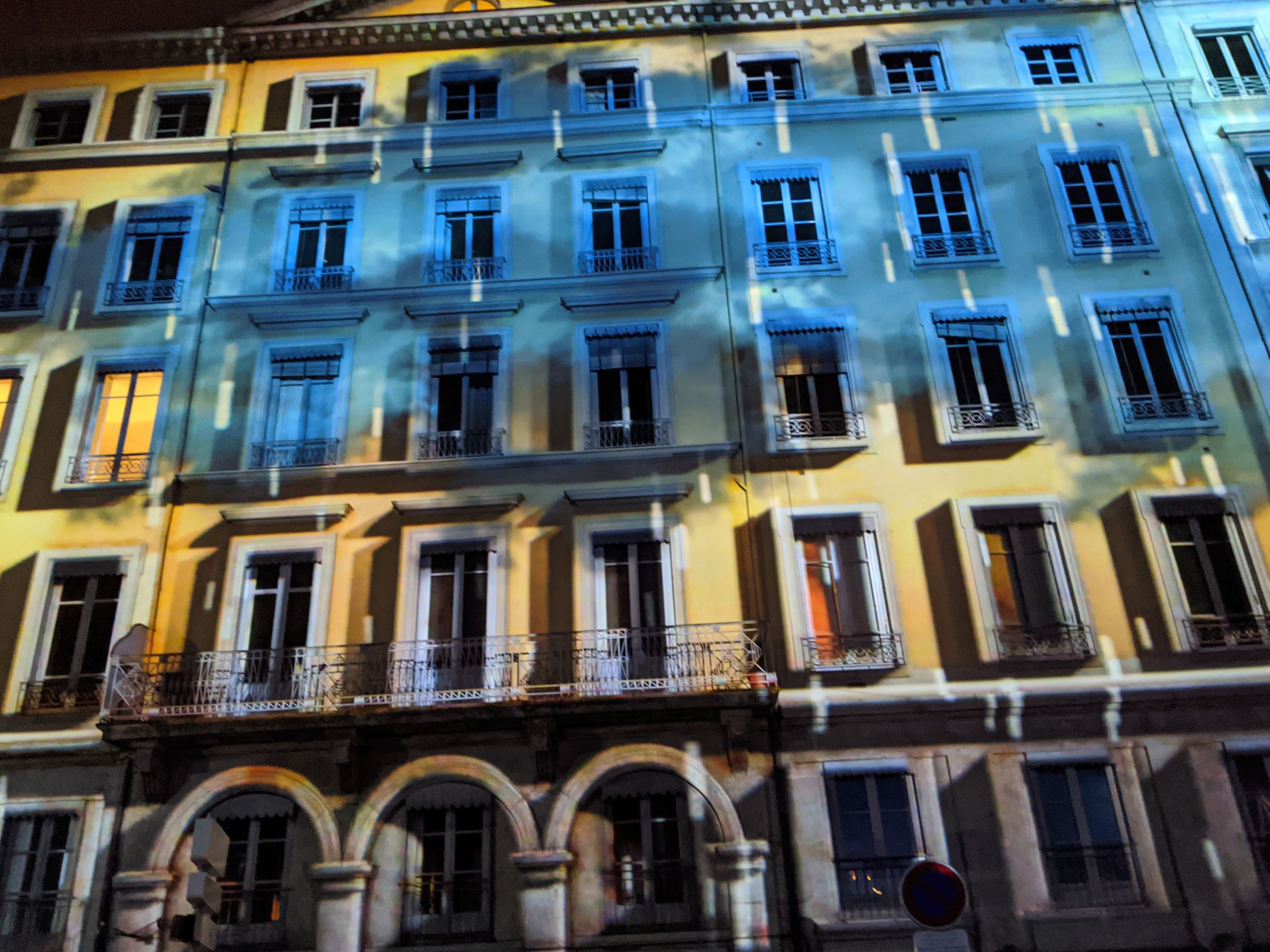
facade.png (original)
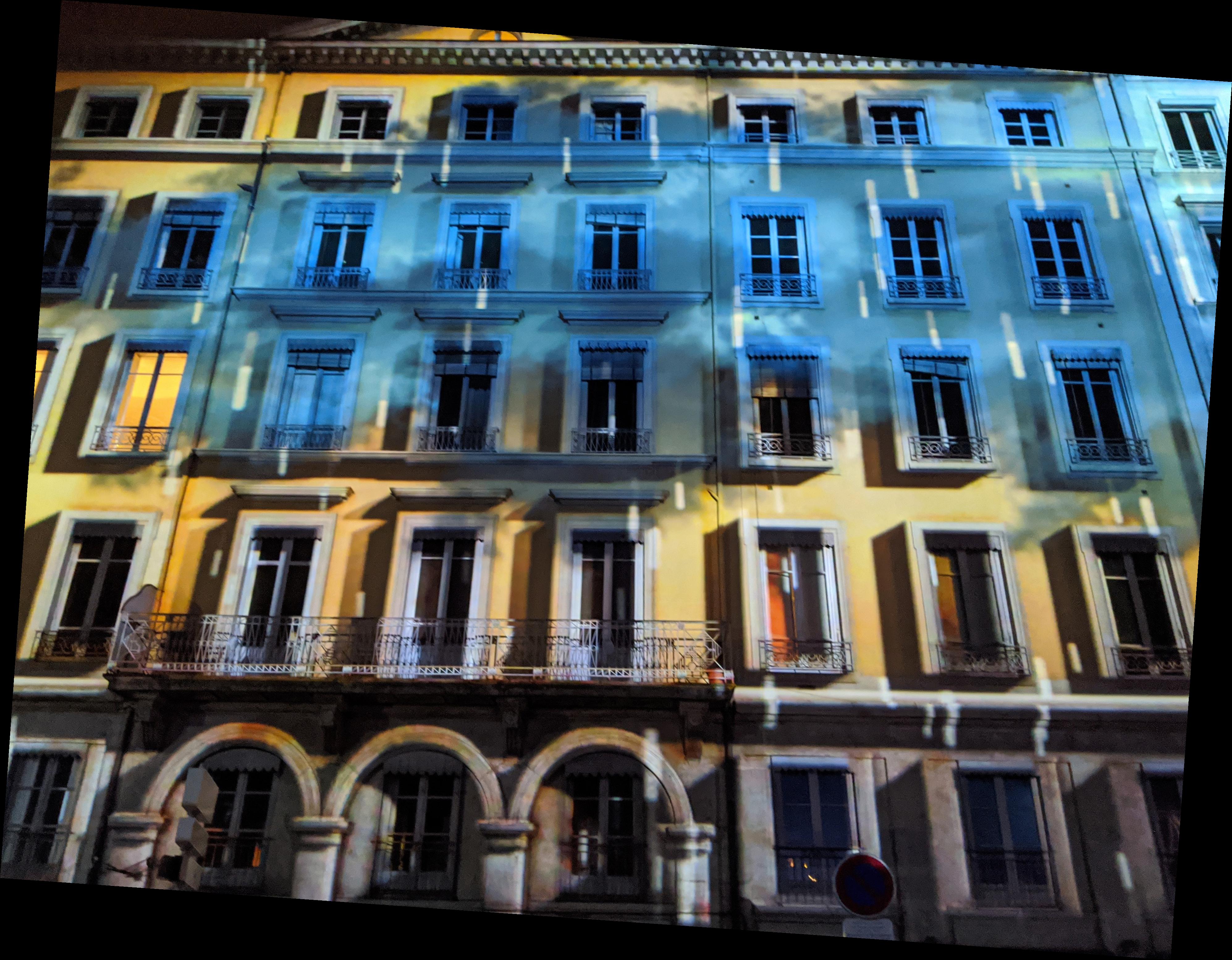
facade.png (rotated -4 degrees)
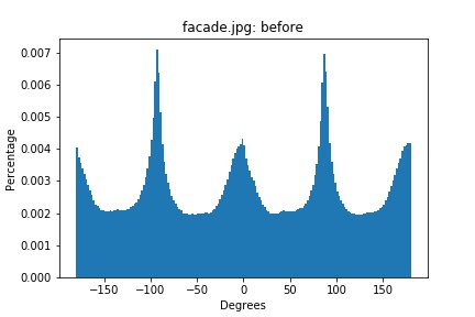
facade.png histogram (original)
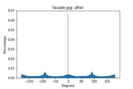
facade.png histogram (rotated -4 degrees)
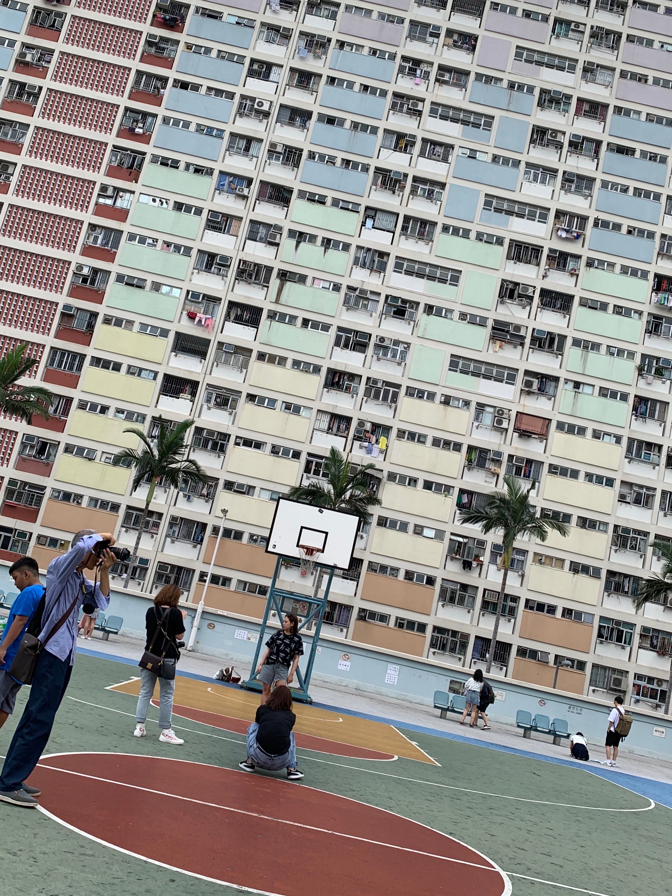
basketball.png (original)
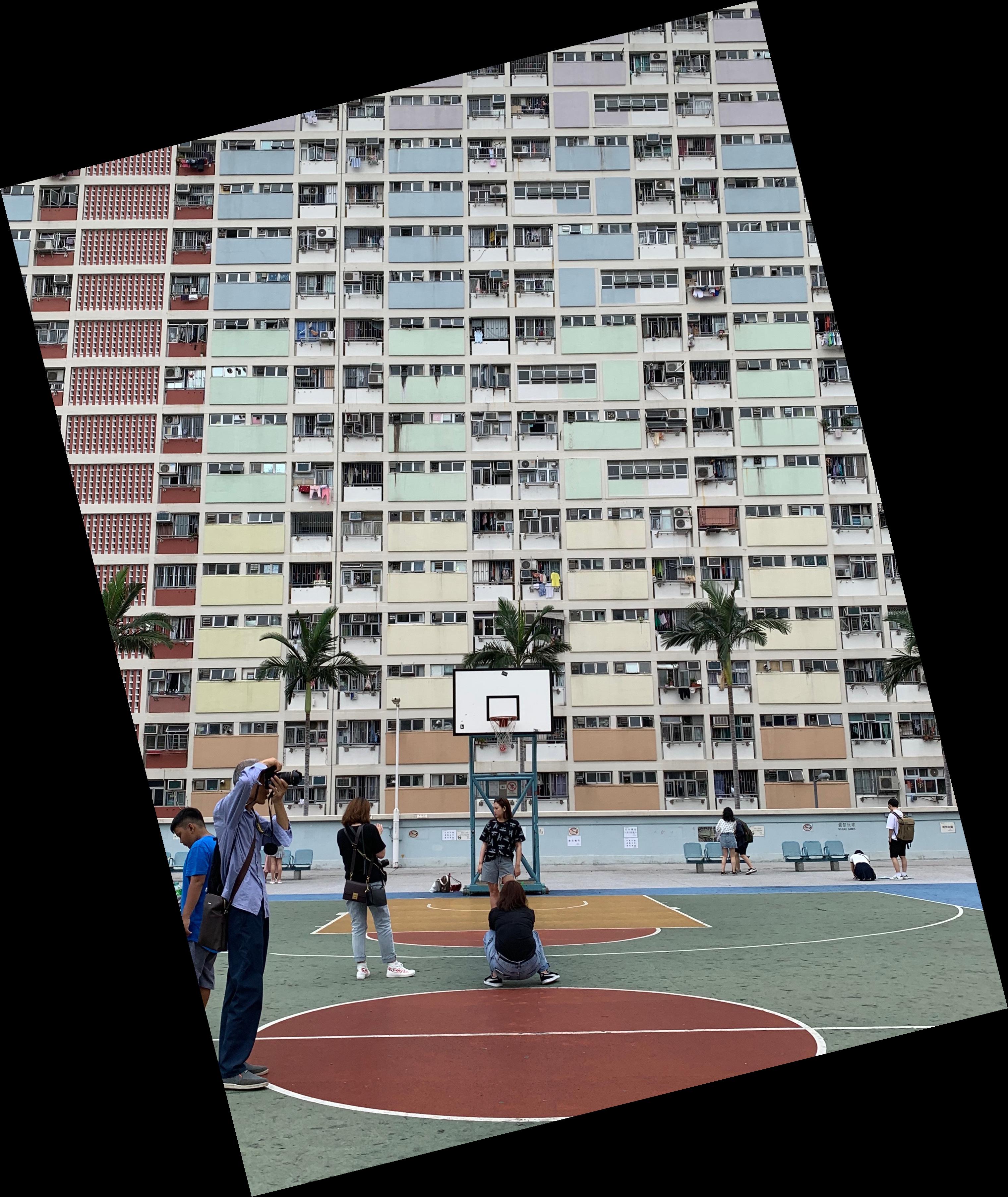
basketball.png (rotated 14 degrees)
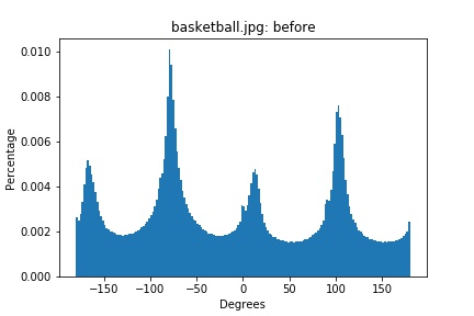
basketball.png histogram (original)
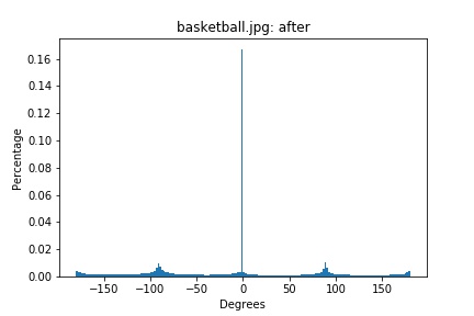
basketball.png histogram (rotated 14 degrees)
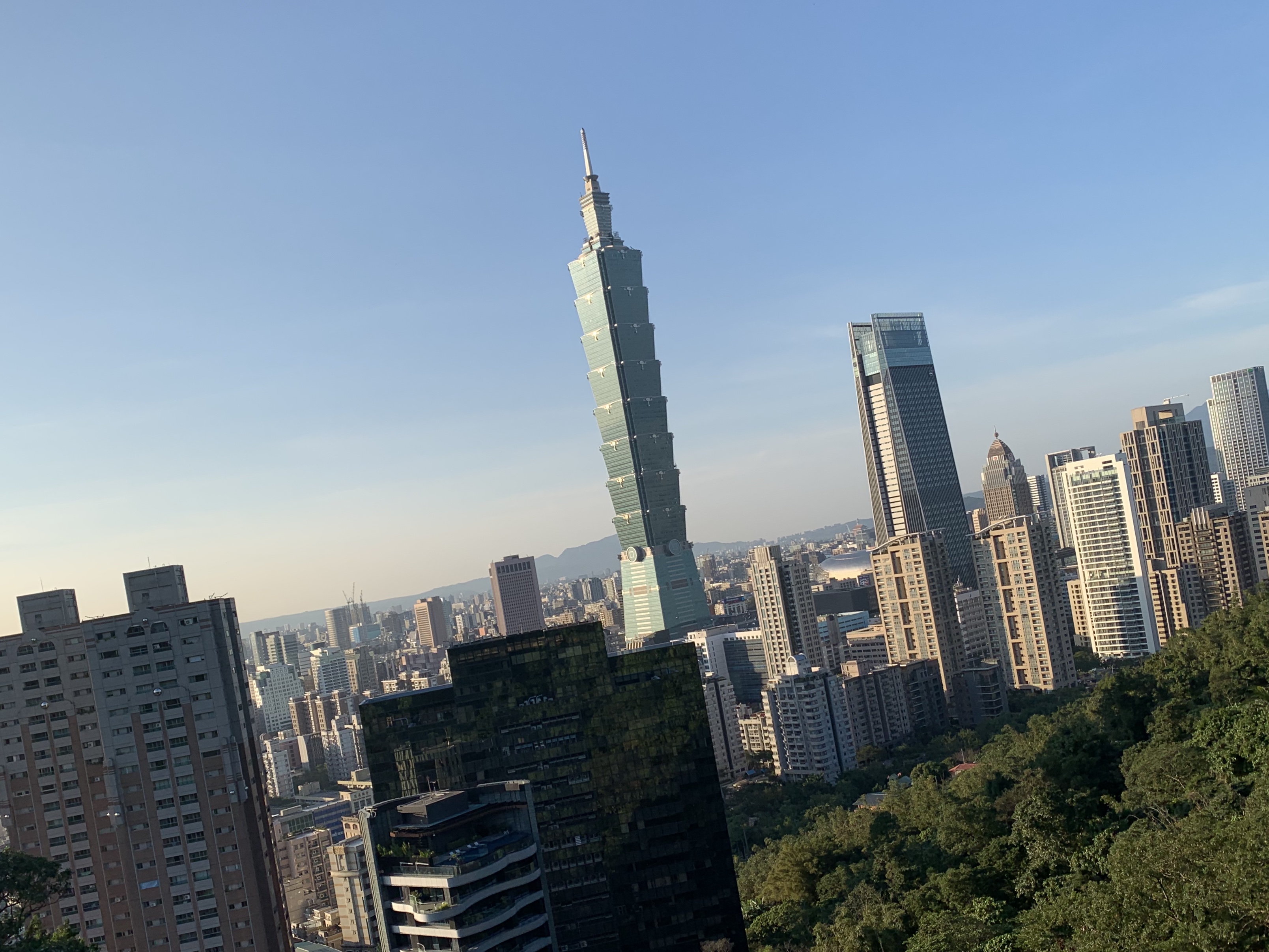
taipei.png (original)
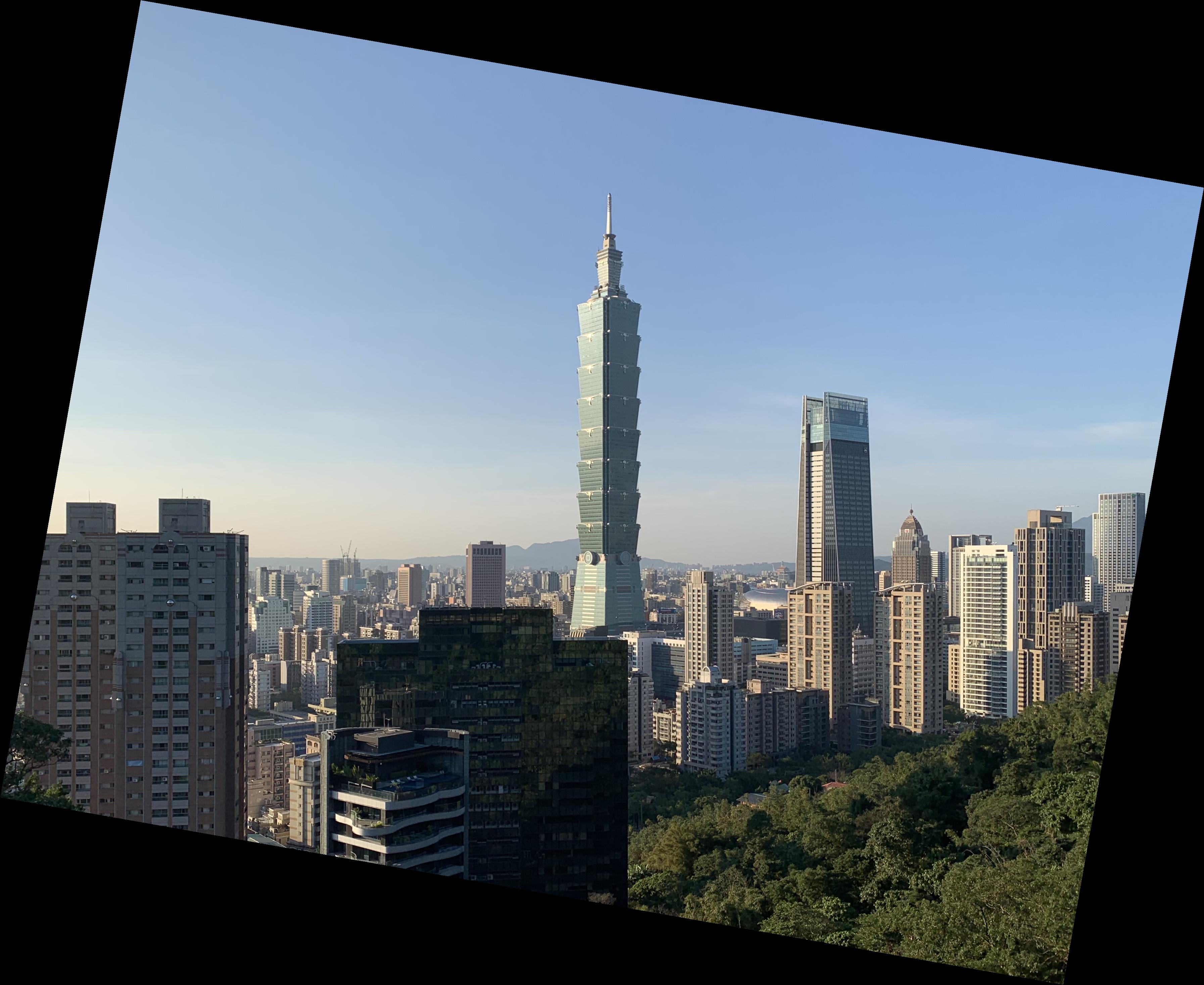
taipei.png (rotated -10 degrees)
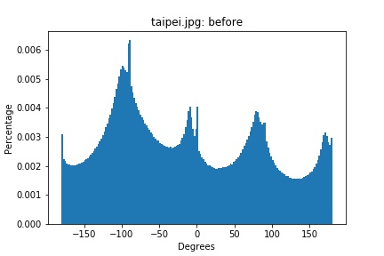
taipei.png histogram (original)
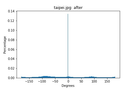
taipei.png histogram (rotated -10 degrees)
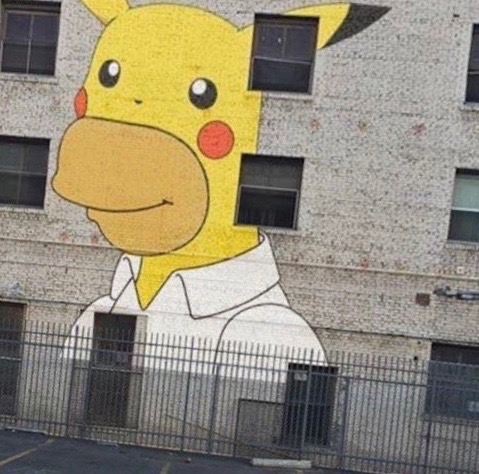
homerchu.png (original)
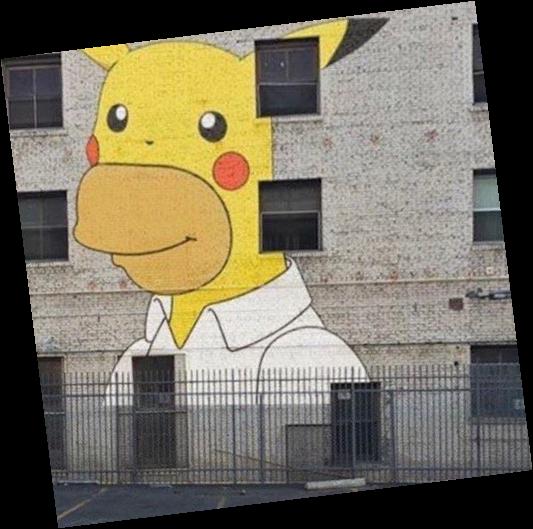
homerchu.png (rotated 7 degrees)
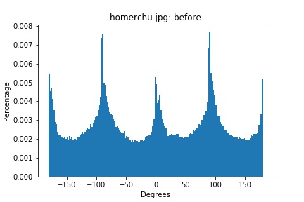
homerchu.png histogram (original)
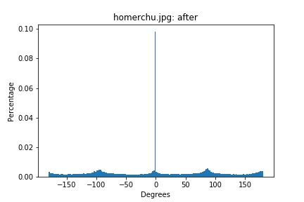
homerchu.png histogram (rotated 7 degrees)
The straightening algorithm fails to straighten the bottom picture most likely because the most distinctive lines (the different colored flowers) should not actually be straight. The algorithm tries to straighten these lines, which results in a originally straight picture now rotated.
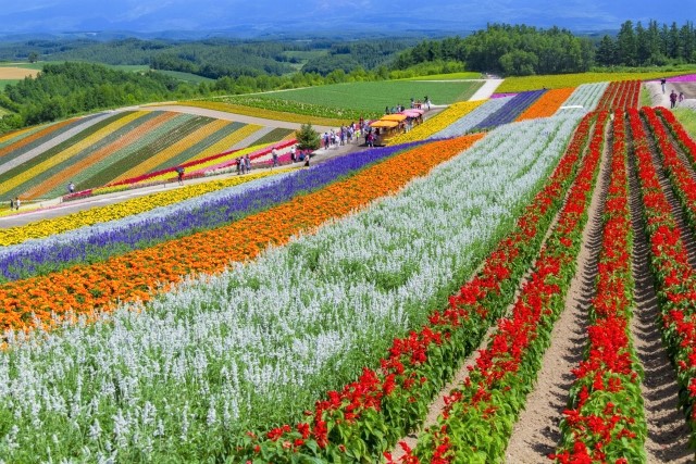
sapporo.png (original)
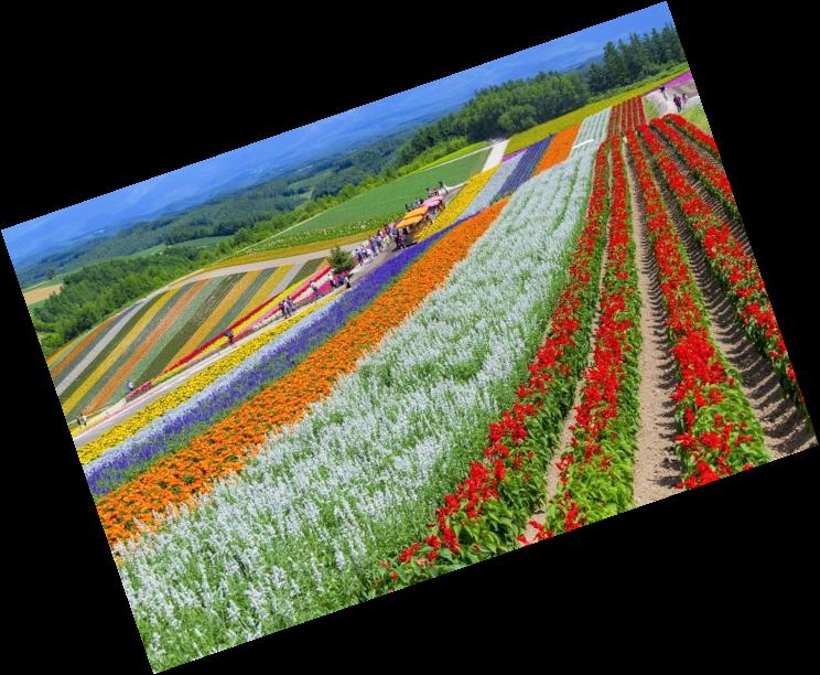
sapporo.png (rotated 19 degrees)
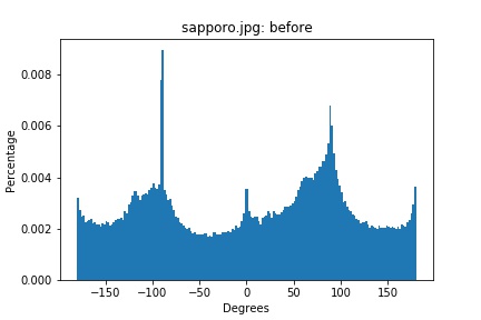
sapporo.png histogram (original)
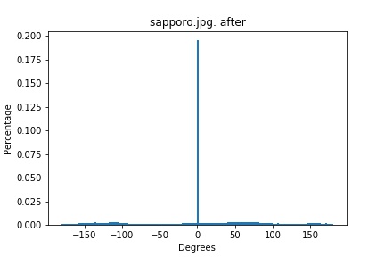
sapporo.png histogram (rotated 19 degrees)
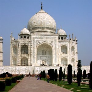
taj.png (original)
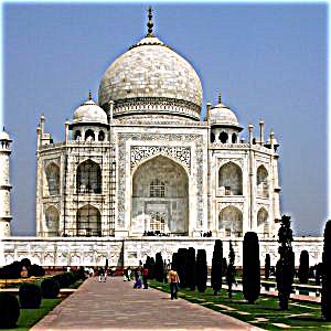
taj.png (sharpened)
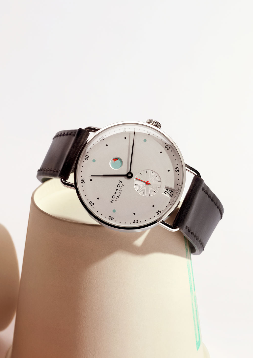
nomos.png (original)
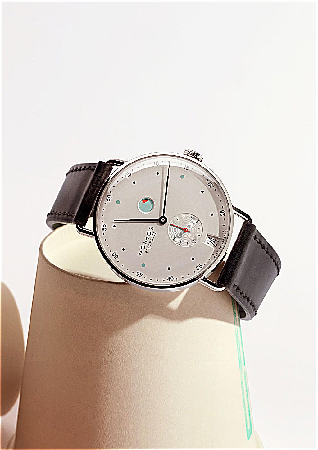
nomos.png (sharpened)
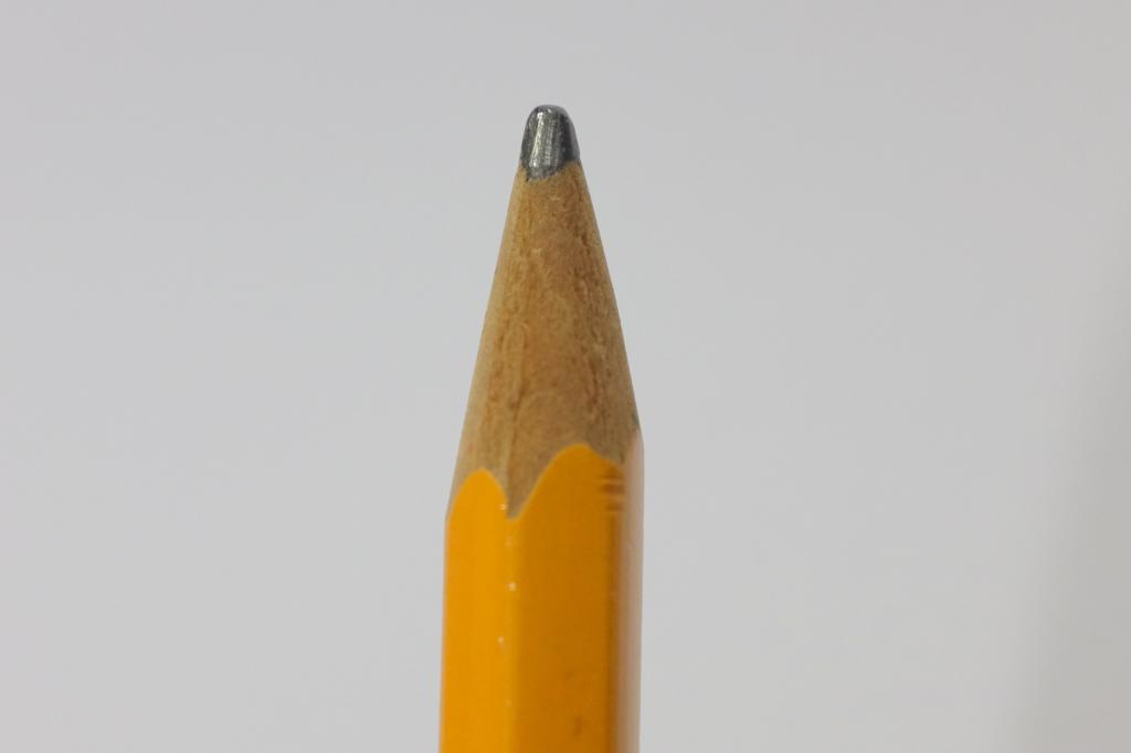
pencil.png (original)
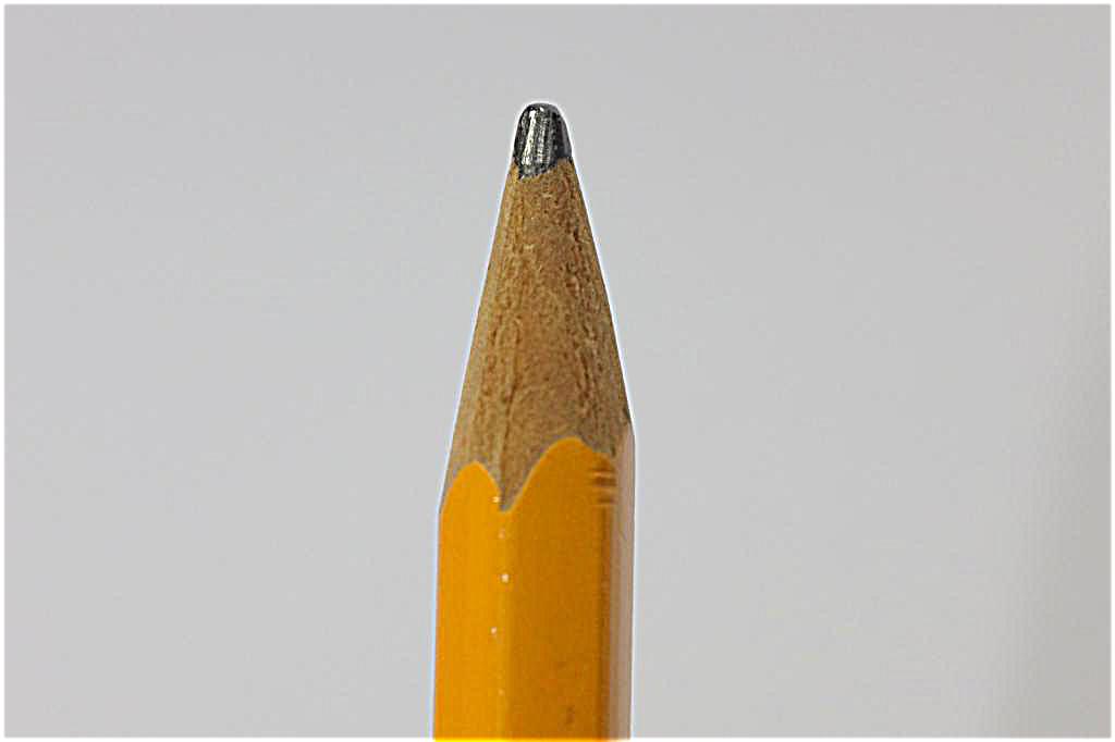
pencil.png (sharpened)

yosemite.png (original)
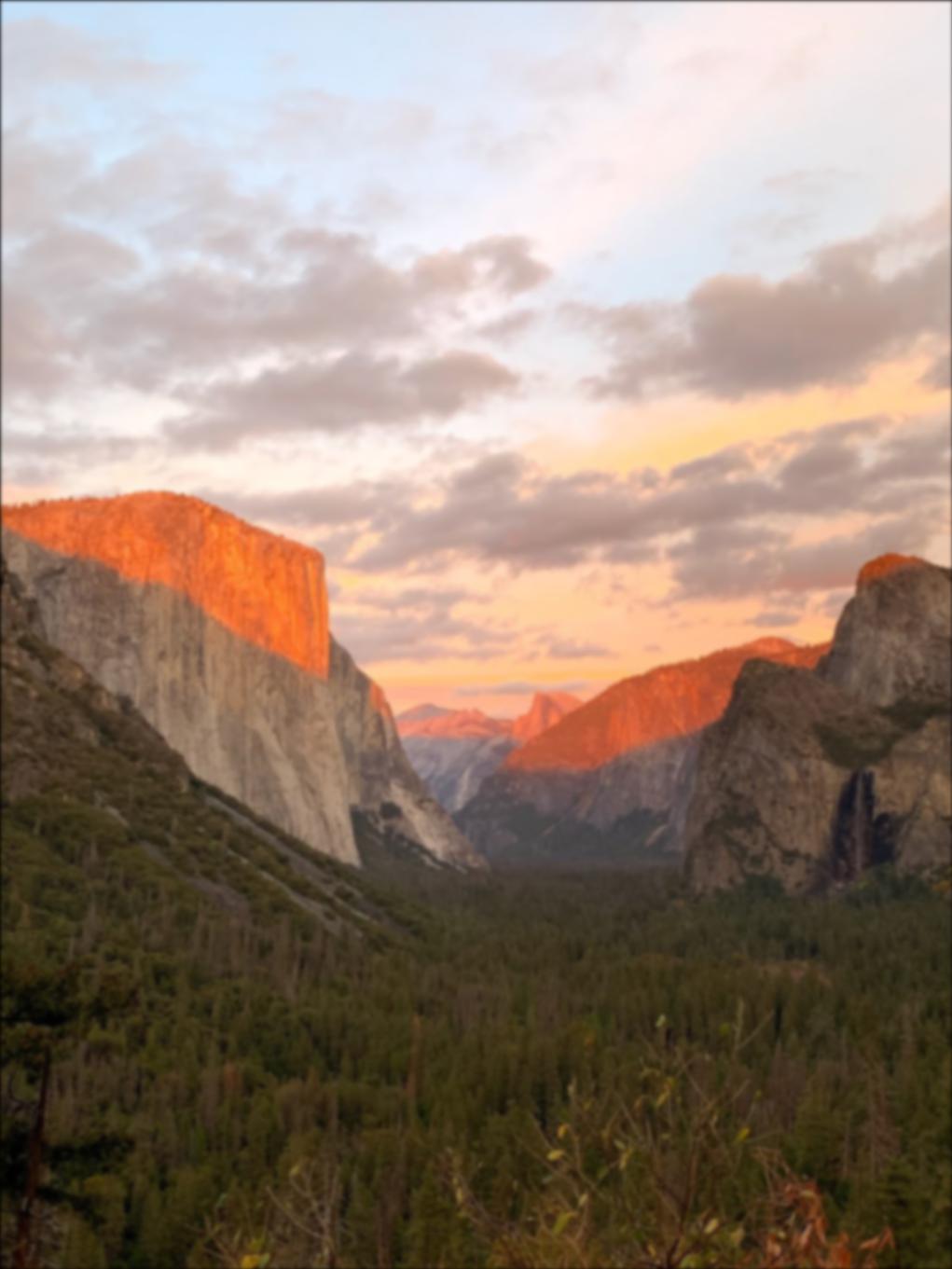
yosemite.png (blurred)
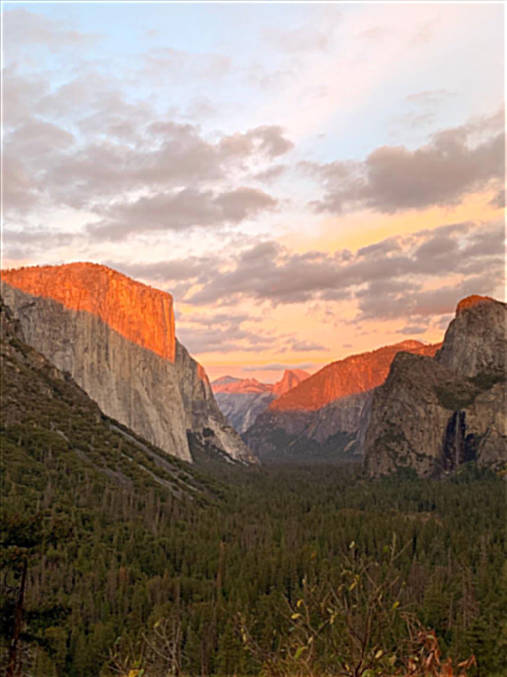
yosemite.png (sharpened)
yosemite.png (original)
Grayscale Images:
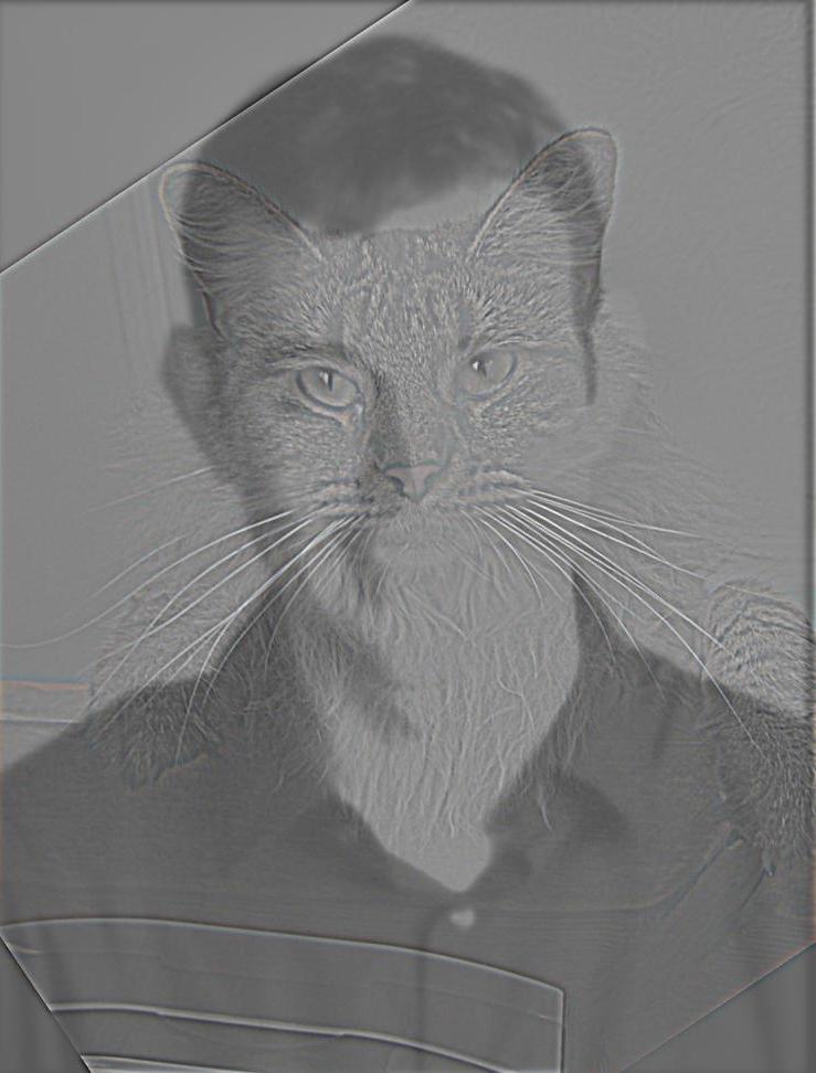
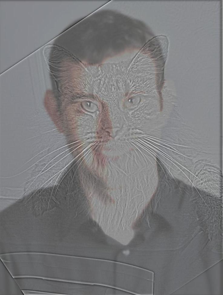
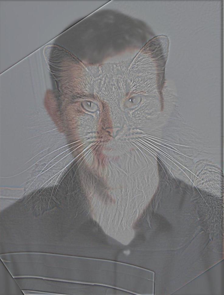
nutmeg.png (original)
DerekPicture.png (original)
nutmeg-derek.png (hybrid)
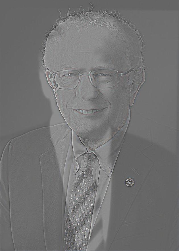
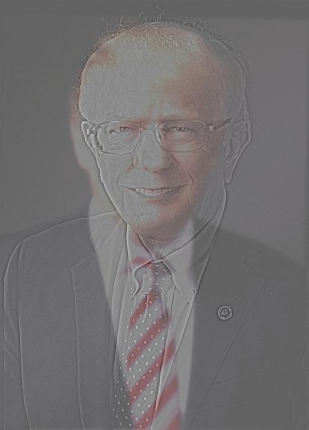
sanders.png (original)
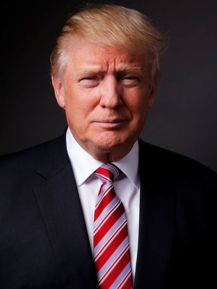
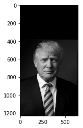
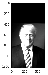
trump.png (original)
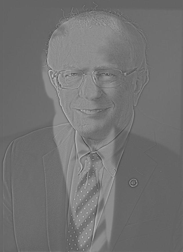
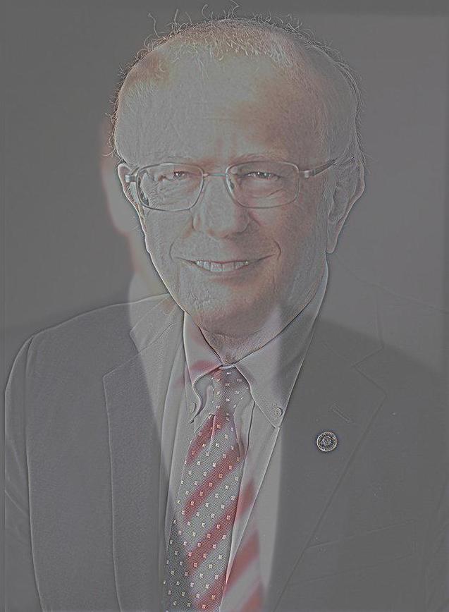
sanders-trump.png (hybrid)
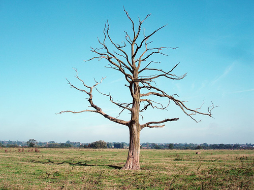
tree_two.png (original)
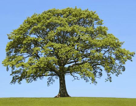
tree_one.png (original)
tree-blend.png (hybrid)
mic.png (original)
dandelion.png (original)
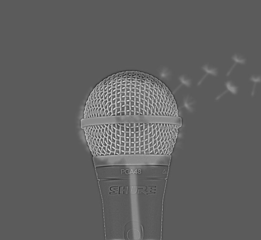
mic-dandelion.png (hybrid)
Failure Case: (SF and NYC skylines). I think this failed because there are a lot of small and indistinct edges from the buildings. Also for the NYC skyline, a lot of the buildings are glass, which reflects the color of the sky and makes the edge between them less distinctive. The blurring effect thus looks stronger and when the two skylines are combined only the high frequency lines are seen.
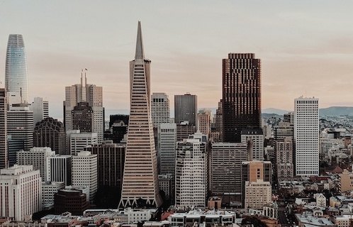
sf.png (original)
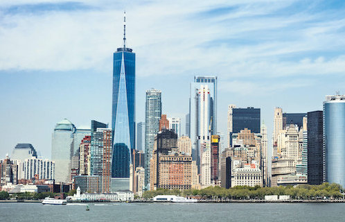
newyork.png (original)
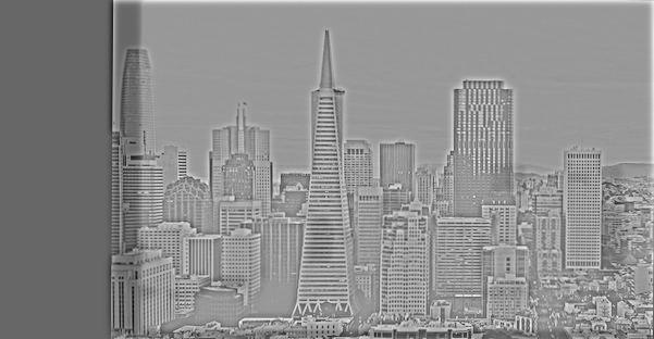
sf-newyork.png (hybrid)
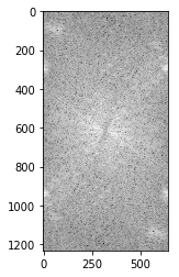
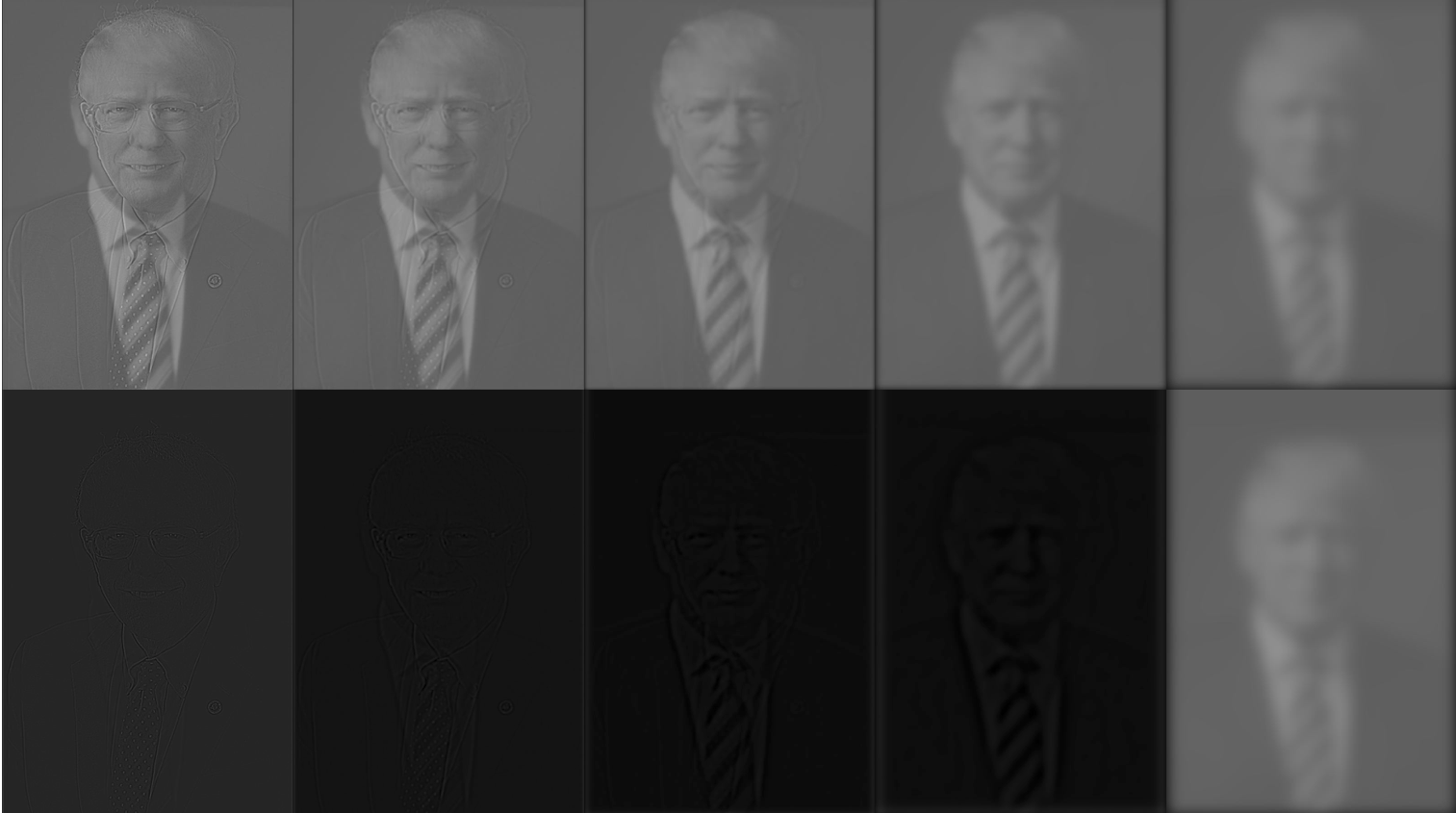
FFT Analysis: (sanders + trump)
Sanders (grayscale) frequency
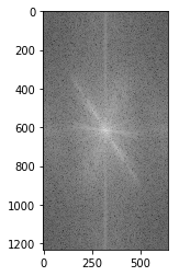
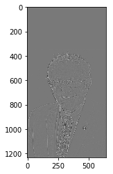
Trump (grayscale) frequency
Sanders frequency (high freq only)
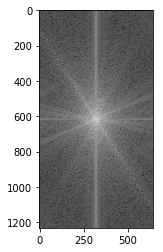
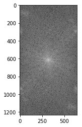
Trump frequency (low freq only)
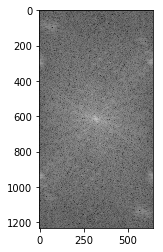
Hybrid frequency
Bells and Whistles: (colored images). There is just a subtle difference when adding the color for the high frequency portion. I think the having color for both images looks the best.
nutmeg-derek.png
nutmeg-derek-nutmeg-color.png
nutmeg-derek-derek-color.png
nutmeg-derek-full-color.png
sanders-trump.png
sanders-trump-sanders-color.png
sanders-trump-trump-color.png
sanders-trump-full-color.png
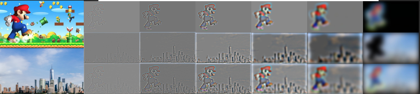
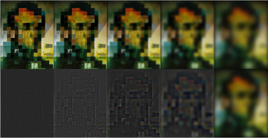
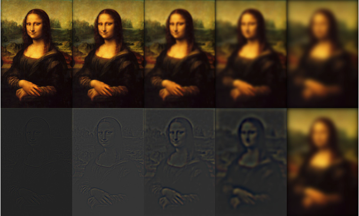
Each top row shows the gaussian stack for sigma=1,2,4,8,16 and size=2*sigma. The bottom row shows the corresponding laplacian stack of the iamge.
lincoln.png
monalisa.png
sanders-trump.png
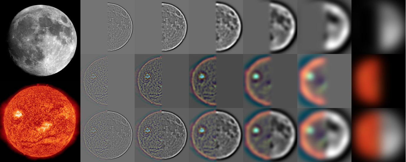
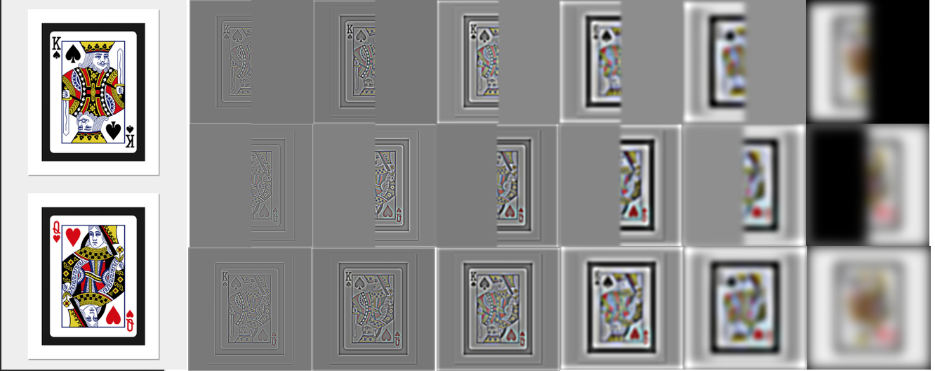
Each blended image has the two original images on the left, followed by the laplacian stack of the first image weighted by the gaussian stack of the mask (top row), the laplacian stack of the second image weighted by the gaussian stack of the mask (middle row), followed by combination of the top and middle row (bottom row). The final blended image is right below.
The following images are blended using a vertical mask:

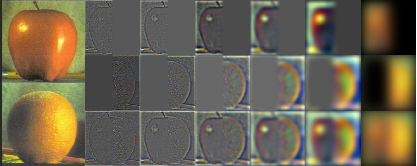
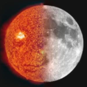
Oraple
Soon
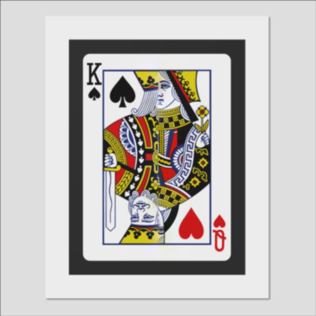
Kueen
The images below are blended using an irregular mask:
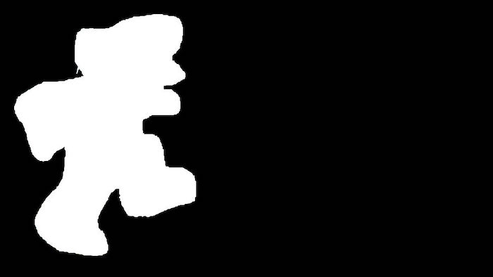
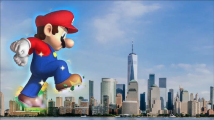
Mario in NYC